Deep Learning
This session will get you started with TensorFlow for R. The best place to get started with TensorFlow is using Keras - a Deep Learning API created by François Chollet and ported to R by JJ Allaire. Keras makes it easy to get started, and it allows you to progressively build more complex workflows as you need to use advanced models and techniques.
Theory Input
For those unfamiliar with Neural Networks, read this article. It’s very comprehensive, and you’ll leave with a general understanding of the types of deep learning and how they work.
There are good reasons to get into deep learning: Deep learning has been outperforming the respective “classical” techniques in areas like image recognition and natural language processing for a while now, and it has the potential to bring interesting insights even to the analysis of tabular data.
Tensorflow
TensorFlow is an end-to-end open-source platform for machine learning. It’s a comprehensive and flexible ecosystem of tools, libraries and other resources that provide workflows with high-level APIs. The framework offers various levels of concepts for you to choose the one you need to build and deploy machine learning models. TensorFlow was originally developed by researchers and engineers working on the Google Brain team within Google’s Machine Intelligence Research organization to conduct machine learning and deep neural networks research.
Keras
The easiest way to get started with Tensorflow is using the Keras API. It is a high-level, declarative way of specifying a model, training and testing it. It enables fast experimation. Being able to go from idea to result with the least possible delay is key to doing good research. Keras has the following key features:
- Allows the same code to run on CPU or on GPU, seamlessly.
- User-friendly API which makes it easy to quickly prototype deep learning models.
- Built-in support for convolutional networks (for computer vision), recurrent networks (for sequence processing), and any combination of both.
- Supports arbitrary network architectures: multi-input or multi-output models, layer sharing, model sharing, etc. This means that Keras is appropriate for building essentially any deep learning model, from a memory network to a neural Turing machine.
See the main Keras website at https://keras.io for additional information on the project.
Before running using keras you need to have it installed. The Keras R interface uses the TensorFlow backend engine by default.
install.packages("keras")
library(keras)
Building a deep Learning Model
We’re going to build a special class of ANN called a Multi-Layer Perceptron (MLP). MLPs are one of the simplest forms of deep learning, but they are both highly accurate and serve as a jumping-off point for more complex algorithms. MLPs are quite versatile as they can be used for regression, binary and multi classification (and are typically quite good at classification problems).
Let’s walk-through the steps before we implement in R.
- Initialize a sequential model: The first step is to initialize a sequential model with
keras_model_sequential(), which is the beginning of our Keras model. The sequential model is composed of a linear stack of layers. - Apply layers to the sequential model: Layers consist of the input layer, hidden layers and an output layer. The input layer is the data and provided it’s formatted correctly there’s nothing more to discuss. The hidden layers and output layers are what controls the ANN inner workings.
- Hidden Layers: Hidden layers form the neural network nodes that enable non-linear activation using weights. The hidden layers are created using
layer_dense(). We’ll add two hidden layers in the business case and the challenge. These parameters can be optimized through hyperparameter tuning. - Dropout Layers: Dropout layers are used to control overfitting. This eliminates weights below a cutoff threshold to prevent low weights from overfitting the layers.
- Output Layer: The output layer specifies the shape of the output and the method of assimilating the learned information. The output layer is applied using the
layer_dense(). For binary values, the shape should be units = 1. For multi-classification, the units should correspond to the number of classes.
- Compile the model: The last step is to compile the model with
compile(). We’ll useoptimizer = "adam", which is one of the most popular optimization algorithms. We select loss =binary_crossentropyfor a binary classification problem andsparse_categorical_crossentropywhen there are two or more label classes. See here for other loss functions. We’ll selectmetrics = c("accuracy")to be evaluated during training and testing.
Business case
In this first business case, we will train a neural network model to classify images of clothing, like sneakers and shirts. It’s fine if you don’t understand all the details, this is a fast-paced overview of a complete Keras program with the details explained as we go.
Data
This guide uses the Fashion MNIST dataset of Zalando’s article images — consisting of a training set of 60,000 examples and a test set of 10,000 examples. The images show individual articles of clothing (10 categories) at low resolution (grayscale, 28 by 28 pixels), as seen here:
We will use 60,000 images to train the network and 10,000 images to evaluate how accurately the network learned to classify images. You can access the Fashion MNIST directly from Keras:
fashion_mnist <- dataset_fashion_mnist()

c(train_images, train_labels) %<-% fashion_mnist$train
c(test_images, test_labels) %<-% fashion_mnist$test

# Notice: Multiple assignment operator was used
# ?'%<-%'
# Is identical to:
# train_images <- fashion_mnist$train$x
# train_labels <- fashion_mnist$train$y
Alternatively, you can clone the zalandoresearch/fashion-mnist GitHub repository or download it here:
| Name | Content | Examples | Size | Link |
|---|---|---|---|---|
| train-images-idx3-ubyte.gz | training set images | 60.000 | 26 MBytes | Download |
| train-labels-idx1-ubyte.gz | training set labels | 60.000 | 29 KBytes | Download |
| t10k-images-idx3-ubyte.gz | test set images | 10.000 | 4,3 MBytes | Download |
| t10k-labels-idx1-ubyte.gz | test set labels | 10.000 | 5,1 KBytes | Download |
At this point we have four arrays: The train_images and train_labels arrays are the training set — the data the model uses to learn. The model is tested against the test set: the test_images, and test_labels arrays.
The images each are 28 x 28 arrays, with pixel values ranging between 0 and 255. The labels are arrays of integers, ranging from 0 to 9. These correspond to the class of clothing the image represents:
| Label | Description |
|---|---|
| 0 | T-Shirt/top |
| 1 | Trouser |
| 2 | Pullover |
| 3 | Dress |
| 4 | Coat |
| 5 | Sandal |
| 6 | Shirt |
| 7 | Sneaker |
| 8 | Bag |
| 9 | Ankle boot |
Each image is mapped to a single label. Since the class names are not included with the dataset, we’ll store them in a vector to use later when plotting the images.
class_names = c("T-shirt/top",
                "Trouser",
                "Pullover",
                "Dress",
                "Coat",
                "Sandal",
                "Shirt",
                "Sneaker",
                "Bag",
                "Ankle boot")
Explore the data
Let’s explore the format of the dataset before training the model. The following shows there are 60.000 [10.000] images in the training set [test set], with each image represented as 28 x 28 pixels. Likewise, there are 60.000 [10.000] labels in the training set [test set]:
dim(train_images)
## [1] 60000    28    28

dim(test_images)
## [1] 10000    28    28

dim(train_labels)
## [1] 60000

dim(test_labels)
## [1] 10000
Each label is an integer between 0 and 9:
train_labels %>%
          unique() %>%
          sort()
## [1] 0 1 2 3 4 5 6 7 8 9
Because the labels are 0-indexed, we have to add always 1 to get the corresponding class_name:
train_labels[1]
## [1] 9

class_names[9 + 1]
## [1] "Ankle boot"
Preprocess the data
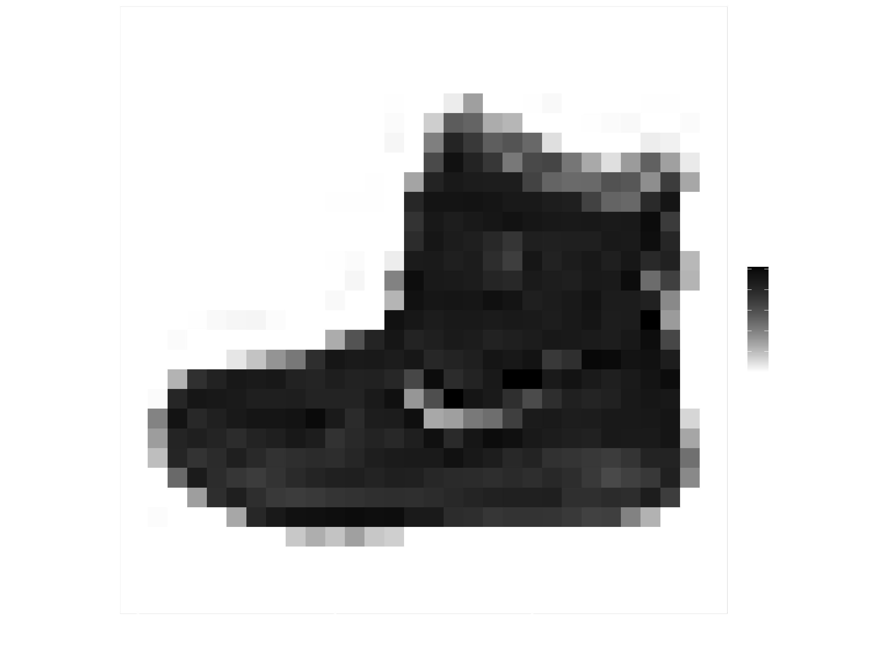
The data must be preprocessed before training the network. If you inspect the first image in the training set, you will see that the pixel values fall in the range of 0 to 255:
library(tidyr)
library(ggplot2)

image_1 <- train_images[1, , ] %>%

                # Convert matrix to a tibble (with unique col names)
                as_tibble(.name_repair = "unique") %>%

                # Set the names according to the col number
                set_names( seq_len(ncol(.)) ) %>%

                # Create a column for the rownumbers
                mutate(y = seq_len(nrow(.))) %>%

                # Make the data long, so that we have x/y value pairs
                pivot_longer(cols = c(1:28), names_to        = "x",
                                             values_to       = "value",
                                             names_transform = list(x = as.integer))

image_1 %>% ggplot(aes(x = x, y = y, fill = value)) +

            # Add tiles and fill them with a white/black gradient
            geom_tile() +
            scale_fill_gradient(low = "white", high = "black", na.value = NA) +

            # Turn image upside down
            scale_y_reverse() +

            # Formatting
            theme_minimal() +
            theme(panel.grid = element_blank()) +
            xlab("") +
            ylab("")
We scale these values to a range of 0 to 1 before feeding to the neural network model. For this, we simply divide by 255.
It’s important that the training set and the testing set are preprocessed in the same way:
train_images <- train_images / 255
test_images  <- test_images / 255
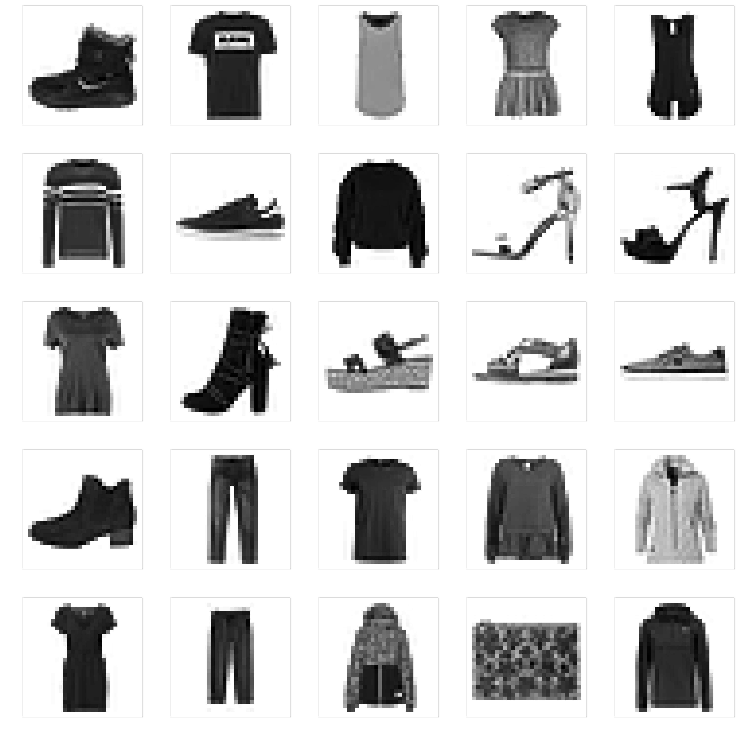
Let’s display the first 25 images from the training set and display the class name below each image to verify that the data is in the correct format and we’re ready to build and train the network.
If we turn the code from above into a plotting function, we can easily plot multiple plots side by side using the cowplot package.
plot_image <- function(idx) {

  image_idx <- train_images[idx, , ] %>%
                as_tibble(.name_repair = "unique") %>%
                set_names(seq_len(ncol(.))) %>%
                mutate(y = seq_len(nrow(.))) %>%
                pivot_longer(cols = c(1:28), names_to        = "x",
                                             values_to       = "value",
                                             names_transform = list(x = as.integer))

    g     <- image_idx %>%
              ggplot(aes(x = x, y = y, fill = value)) +
              geom_tile() +
              scale_fill_gradient(low = "white", high = "black", na.value = NA) +
              scale_y_reverse() +
              theme_minimal() +
              theme(panel.grid = element_blank(),
                    legend.position = "none",
                    axis.text = element_blank()) +

              # Add the label (add 1, because it is 0-indexed)
              xlab(class_names[train_labels[idx] + 1]) +
              ylab("")

      return(g)

}

library(cowplot)
image_lst <- map(c(1:25), plot_image)
plot_grid(plotlist = image_lst)
Build the model
Building the neural network requires configuring the layers of the model, then compiling the model.
Setup the layers
The basic building block of a neural network is the layer. Layers extract representations from the data fed into them. And, hopefully, these representations are more meaningful for the problem at hand.
Most of deep learning consists of chaining together simple layers. Most layers, like layer_dense, have parameters that are learned during training.
model <- keras_model_sequential()
model %>%
  layer_flatten(input_shape = c(28, 28)) %>%
  layer_dense(units = 128, activation = 'relu') %>%
  layer_dense(units = 10, activation = 'softmax')
The first layer in this network, layer_flatten, transforms the format of the images from a 2d-array (of 28 by 28 pixels), to a 1d-array of 28 * 28 = 784 pixels. Think of this layer as unstacking rows of pixels in the image and lining them up. This layer has no parameters to learn; it only reformats the data.
After the pixels are flattened, the network consists of a sequence of two dense layers. These are densely-connected, or fully-connected, neural layers. The first dense layer has 128 nodes (or neurons). The second (and last) layer is a 10-node softmax layer —this returns an array of 10 probability scores that sum to 1. Each node contains a score that indicates the probability that the current image belongs to one of the 10 digit classes.
Compile the model
Before the model is ready for training, it needs a few more settings. These are added during the model’s compile step:
Loss function: This measures how accurate the model is during training. We want to minimize this function to “steer” the model in the right direction.Optimizer: This is how the model is updated based on the data it sees and its loss function.Metrics: Used to monitor the training and testing steps. The following example uses accuracy, the fraction of the images that are correctly classified.
model %>% compile(
  optimizer = 'adam',
  loss = 'sparse_categorical_crossentropy',
  metrics = c('accuracy')
)
Train the mdoel
Training the neural network model requires the following steps:
- Feed the training data to the model — in this example, the
train_imagesandtrain_labelsarrays. - The model learns to associate images and labels.
- We ask the model to make predictions about a test set — in this example, the test_images array. We verify that the predictions match the labels from the test_labels array.
To start training, call the fit method — the model is “fit” to the training data:
model %>% fit(train_images, train_labels, epochs = 5, verbose = 2)
## Epoch 1/5
## 1875/1875 - 3s - loss: 0.5003 - accuracy: 0.8231
## Epoch 2/5
## 1875/1875 - 5s - loss: 0.3770 - accuracy: 0.8632
## Epoch 3/5
## 1875/1875 - 2s - loss: 0.3378 - accuracy: 0.8769
## Epoch 4/5
## 1875/1875 - 2s - loss: 0.3138 - accuracy: 0.8854
## Epoch 5/5
## 1875/1875 - 2s - loss: 0.2960 - accuracy: 0.8912
As the model trains, the loss and accuracy metrics are displayed. This model reaches an accuracy of about 0.89 (or 89%) on the training data.
Evaluate accuracy
Next, compare how the model performs on the test dataset:
score <- model %>% evaluate(test_images, test_labels, verbose = 0)
score
##      loss  accuracy
## 0.3370821 0.8812000
It turns out, the accuracy on the test dataset is a little less than the accuracy on the training dataset. This gap between training accuracy and test accuracy is an example of overfitting. Overfitting is when a machine learning model performs worse on new data than on their training data.
Make Predictions
With the model trained, we can use it to make predictions about some images.
predictions <- model %>% predict(test_images)
Here, the model has predicted the label for each image in the testing set. Let’s take a look at the first prediction:
predictions[1, ]
## [1] 1.604741e-06 3.105908e-07 6.875617e-08 4.231533e-09 1.337077e-07
## [6] 8.460676e-03 1.049293e-06 3.328498e-02 1.070093e-05 9.582404e-01

predictions[1, ] %>% which.max()
## [1] 10
Alternatively, we can also directly get the class prediction:
class_pred <- model %>% predict_classes(test_images)
class_pred[1:20]
## [1] 9 2 1 1 6 1 4 6 5 7 4 5 5 3 4 1 2 2 8 0
So the model is most confident that this image is an ankle boot. And we can check the test label to see this is correct:
test_labels[1]
## [1] 9

class_names[test_labels[1] + 1]
## [1] "Ankle boot"
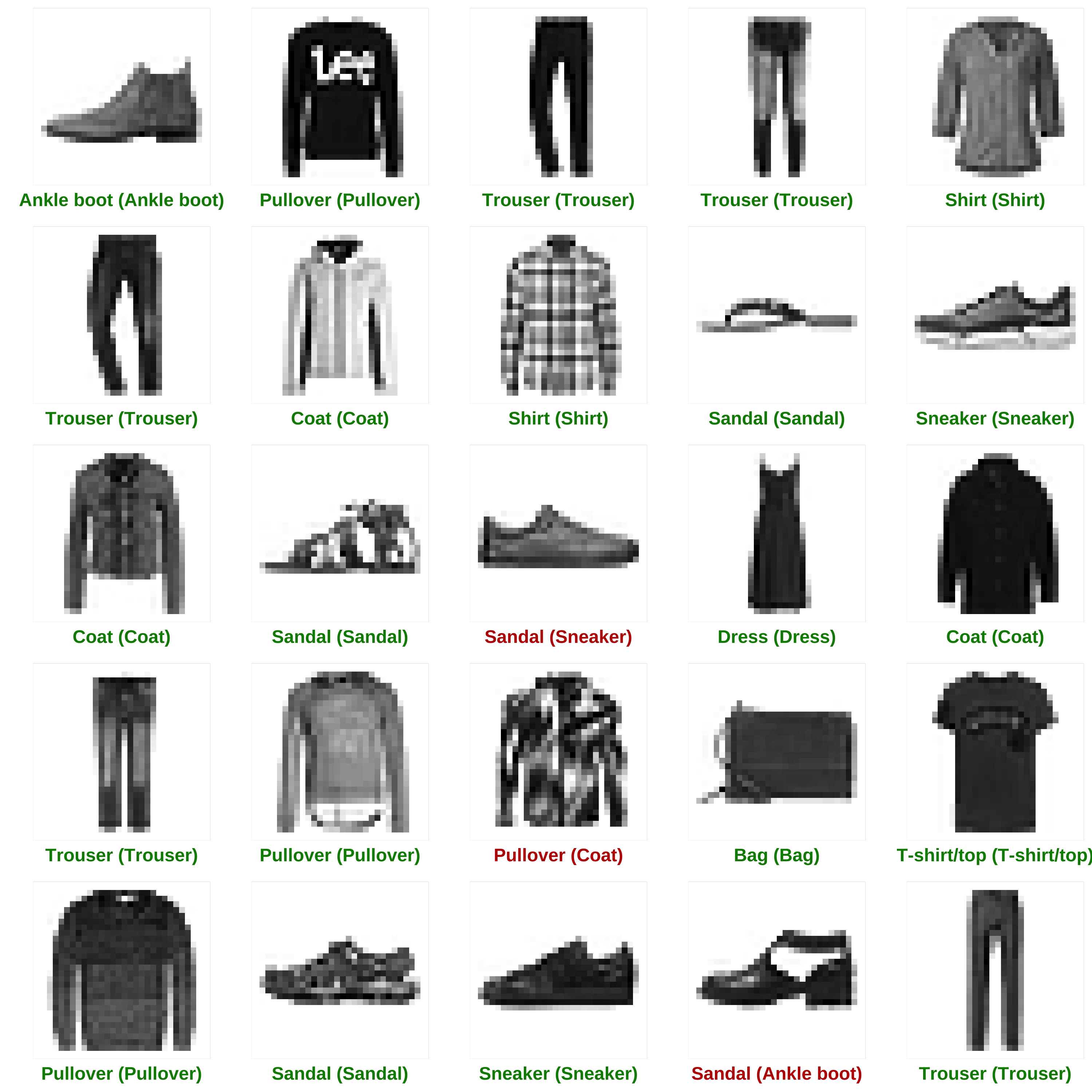
Let’s plot several images with their predictions. Correct prediction labels are green and incorrect prediction labels are red.
## 1. Create function
plot_predictions <- function(idx) {

  # Get image in the correct format
  image_test <- test_images[idx, , ] %>%
                    as_tibble(.name_repair = "unique") %>%
                    set_names( seq_len(ncol(.)) ) %>%
                    mutate(y = seq_len(nrow(.))) %>%
                    pivot_longer(cols = c(1:28),
                                 names_to        = "x",
                                 values_to       = "value",
                                 names_transform = list(x = as.integer))

  # Get true and predicted labels
  # subtract 1 as labels go from 0 to 9
  predicted_label <- which.max(predictions[idx, ]) - 1
  true_label      <- test_labels[idx]
  color           <- ifelse(predicted_label == true_label, "#008800", "#bb0000")

  # Plot
  g <- image_test %>%
          ggplot(aes(x = x, y = y, fill = value)) +
          geom_tile() +
          scale_fill_gradient(low = "white", high = "black", na.value = NA) +
          scale_y_reverse() +
          theme_minimal() +
          theme(panel.grid = element_blank(),
                legend.position = "none",
                axis.text = element_blank(),
                axis.title.x = element_text(color = color, face = "bold")) +
          xlab(paste0(
            class_names[predicted_label + 1],
            " (",
            class_names[true_label + 1], ")")) +
          ylab("")

    return(g)

}

## 2. map over indices
predictions_lst <- map(c(1:25), plot_predictions)

## 3. Plot list
plot_grid(plotlist = predictions_lst)
Finally, use the trained model to make a prediction about a single image.
# Grab an image from the test dataset
# take care to keep the batch dimension, as this is expected by the model -> ?drop
dim(test_images)
## [1] 10000    28    28

img <- test_images[1, , , drop = FALSE]
dim(img)
## [1]  1 28 28
Now predict the image:
predictions <- model %>% predict(img)
predictions
predict() returns an array of lists, one for each image in the batch of data. Grab the predictions for our (only) image in the batch:
which.max(predictions[1, ])
## [1] 10
Or, directly getting the class prediction again:
class_pred <- model %>% predict_classes(img)
class_pred
## [1] 9

class_names[class_pred + 1]
## [1] "Ankle boot"
And, as before, the model predicts a label of 9 (“Ankle Boot”)
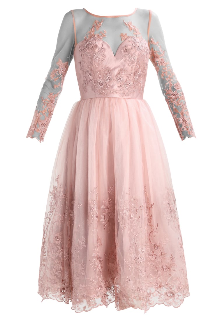
Let’s test our model with a completely new image. First, we have to load the image into R and adjust it to our model. The Zalando dataset consists of Zalando online assortments’ (front-look) photos. Shot by in-house photographers. Class labels were manually annotated by in-house experts.


The processing pipeline includes 7 steps:
- PNG Image
- Trimming
- Resizing
- Sharpening
- Extending
- Negating
- Grayscaling
I have taken the following ( from here):

The steps above translated to a R pipeline:
- Adjust the the pixel size (depth (z) and color (c) can be set to 1, because we want a grayscale image) with
resize() - Rotate by 90 degree with
imrotate() - Convert to array with
as.array() - Remove depth and color dimension with
drop() - Set dimension according to the train and test data
- Invert the color by substracting the values from 1
- We don’t do trimming, resizing, sharpening and extending (meaning the images are not properly cropped and sharpened), but for a first try that should be sufficient.
library(imager)
img_new <- load.image("images/t-shirt.jpg") %>%
resize(size_x = 28, size_y = 28, size_z = 1, size_c = 1) %>%
imrotate(angle = -90) %>%
as.array() %>%
drop() %>%
array(dim = c(1,28,28)) %>%
subtract(1) %>%
abs()
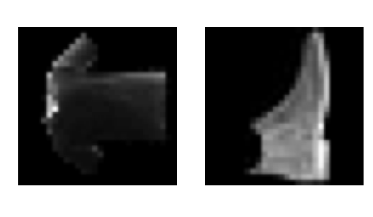
par(mfrow=c(1,2)) # set the plotting area into a 1*2 array
plot(as.cimg(img_new[1,,]), main = "img_new", axes=FALSE)
plot(as.cimg(test_images[1,,]), main = "img_test", axes=FALSE)
The prediction is done analogously:
predictions <- model %>% predict(img_new[1, , , drop = FALSE])
prediction  <- predictions[1, ] - 1
which.max(prediction)
## [1] 1

class_pred <- model %>% predict_classes(img_new)
class_pred
## [1] 0
class_names[class_pred + 1]
## [1] "T-shirt/top"
Challenge
For the challenge we are using tabular data instead of images. The goal is to predict customer churn using deep learning with Keras. The objective is similar to the employee churn prediction from the last session.
Customer churn refers to the situation when a customer ends their relationship with a company, and it’s a costly problem. Customer churn is a problem that all companies need to monitor, especially those that depend on subscription-based revenue streams. Loss of customers impacts sales. We are using the keras package to produce an Artificial Neural Network (ANN) model on the
IBM Watson Telco Customer Churn Data Set! As for most business problems, it’s equally important to explain what features drive the model, which is why we’ll use the lime package for explainability. Moreover, we are going to cross-check the LIME results with a Correlation Analysis.
Credit goes to Susan Li.
We need the following packages:
tidyverse: Loads dplyr, ggplot2 etc. for data wrangling and visualizationkeras: Ports Keras from Python enabling deep learning in Rlime: Used to explain the predictions of black box classifiersrecipes: package for preprocessing machine learning data setsrsample: Package for generating resamplesyardstick: Tidy methods for measuring model performancecorrr: Tidy methods for correlation
According to IBM, the business challenge is…
A telecommunications company [Telco] is concerned about the number of customers leaving their landline business for cable competitors. They need to understand who is leaving. Imagine that you’re an analyst at this company and you have to find out who is leaving and why.
The dataset includes information about:
- Churn: Customers who left within the last month
- Services that each customer has signed up for (phone, internet, steaming, … )
- Customer account information (duration, payment method, … )
- Demographic info about customers (gender, age, … )
Load the libraries and install keras, if you have not installed before:
# Load libraries
library(tidyverse)
library(keras)
library(lime)
library(rsample)
library(recipes)
library(yardstick)
library(corrr)

# Install Keras if you have not installed before
# install_keras()
The entire code is already structured for you. But sometimes there are empty bits (...) which are to be filled by you.
Import the data into a tibble and inspect the data.
churn_data_raw <- ...

glimpse(...)
Preprocess data
First, we “prune” the data, which is nothing more than removing unnecessary columns and rows. The data has a few columns and rows we’d like to remove:
- The “customerID” column is a unique identifier for each observation that isn’t needed for modeling.
- The data has 11 NA values all in the “TotalCharges” column. Because it’s such a small percentage of the total population (99.8% complete cases), we can drop these observations (the
tidyrpackage provides a function for that. Typetidyr::to get a list of the function.) - have the target in the first column
churn_data_tbl <- ... %>%
                  ... %>%
                  ... %>%
                  ...
Split the data into a training and testing dataset (proportion: 80/20)
# Split test/training sets
set.seed(100)
train_test_split <- ...
train_test_split

## <Analysis/Assess/Total>
## <5626/1406/7032>

# Retrieve train and test sets
train_tbl <- ...
test_tbl  <- ...
Exploration: What Transformation Steps Are Needed For ML?
This phase of the analysis is often called exploratory analysis, but basically we are trying to answer the question, “What steps are needed to prepare for ML?” The key concept is knowing what transformations are needed to run the algorithm most effectively. Artificial Neural Networks are best when the data is one-hot encoded, scaled and centered.
Discretize the “tenure” feature
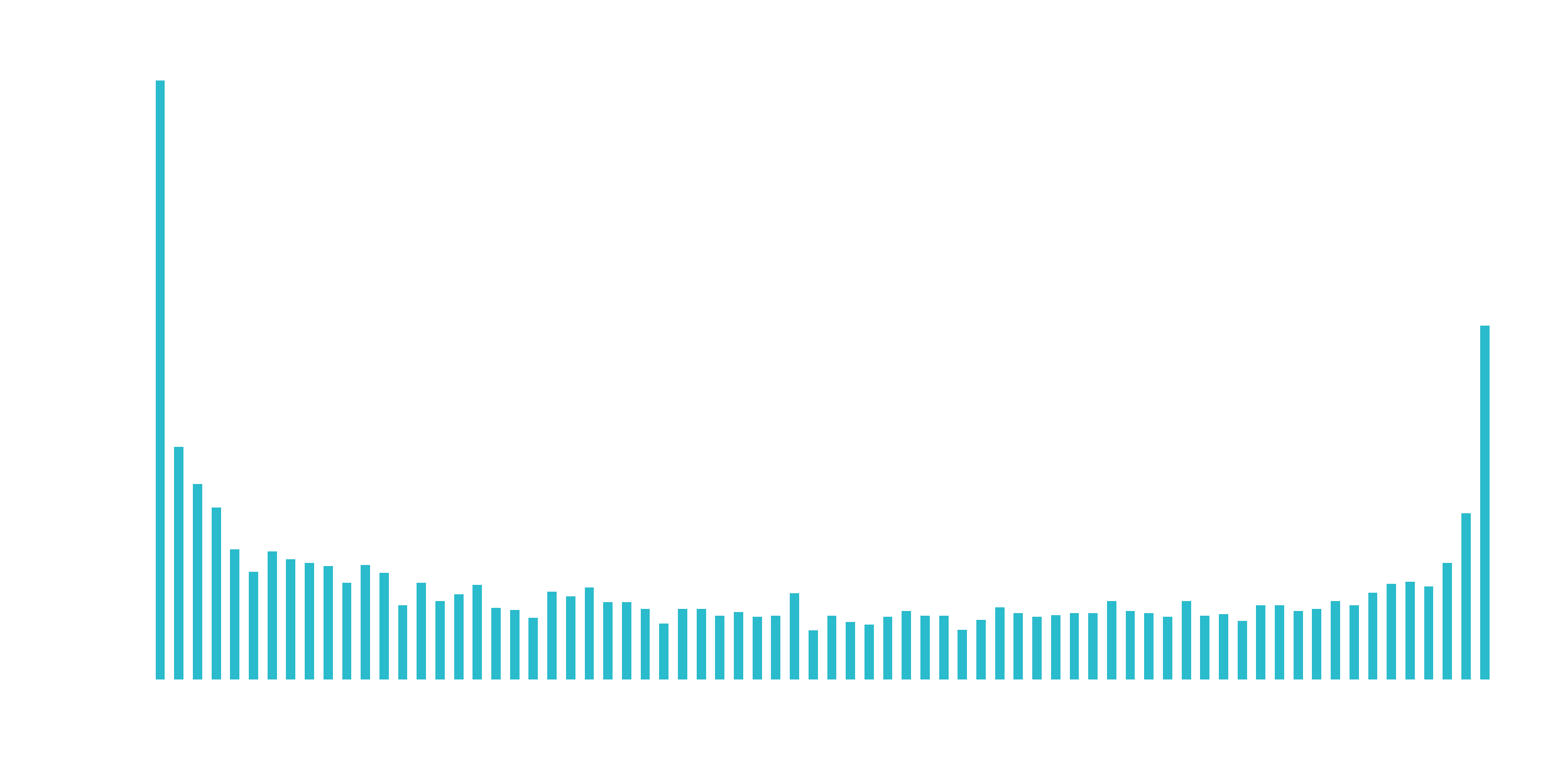
Numeric features like age, years worked, length of time in a position can generalize a group (or cohort). The “tenure” feature falls into this category of numeric features that can be discretized into groups.
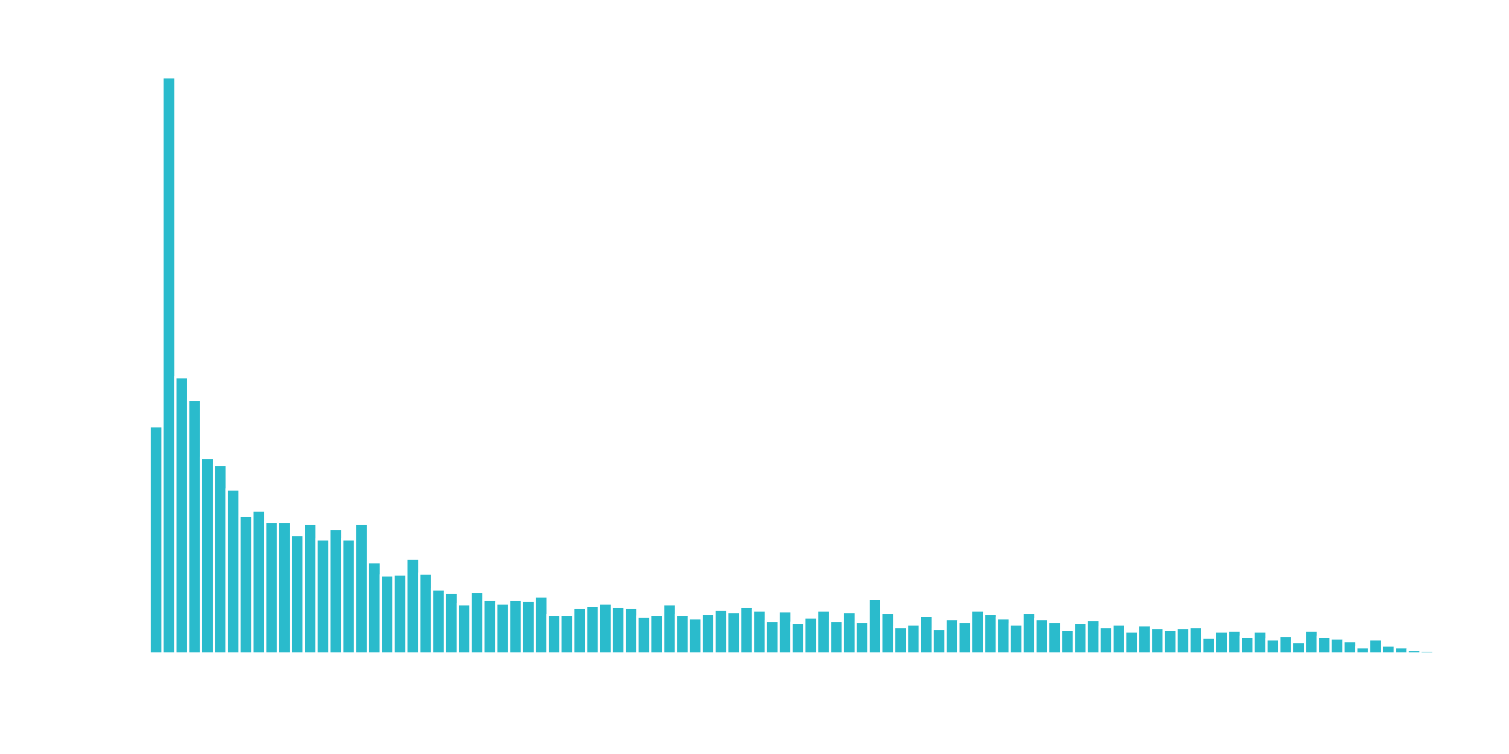
hist(churn_data_tbl)
# churn_data_tbl %>% ggplot(aes(x = tenure)) +
#                       geom_histogram(binwidth = 0.5, fill =  "#2DC6D6") +
#                       labs(
#                         title = "Tenure Counts Without Binning",
#                         x     = "tenure (month)"
#                         )
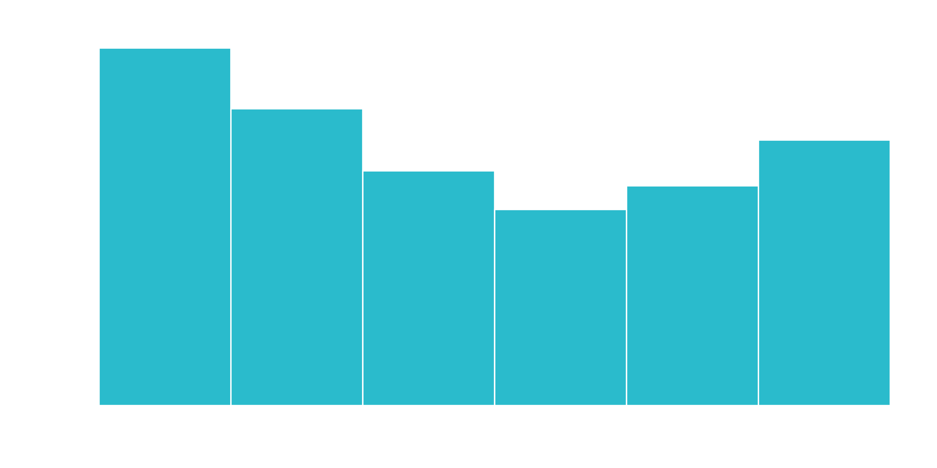
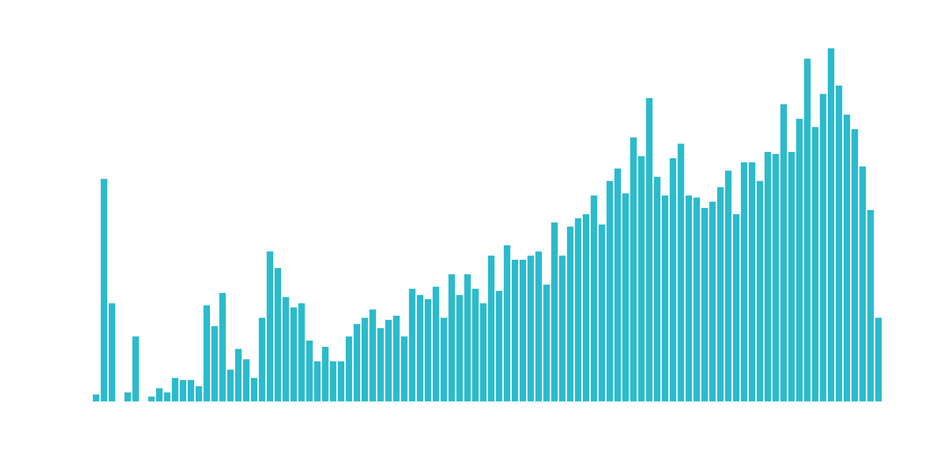
We can split into six cohorts that divide up the user base by tenure in roughly one year (12 month) increments. This should help the ML algorithm detect if a group is more/less susceptible to customer churn.
churn_data_tbl %>% ggplot(aes(x = tenure)) +
  geom_histogram(bins = 6, color = "white", fill =  "#2DC6D6") +
  labs(
    title = "Tenure Counts With Six Bins",
    x     = "tenure (month)"
  )
Transform the “TotalCharges” feature
What we don’t like to see is when a lot of observations are bunched within a small part of the range.
We can use a log transformation to even out the data into more of a normal distribution. It’s not perfect, but it’s quick and easy to get our data spread out a bit more.
A quick test is to see if the log transformation increases the magnitude of the correlation between “TotalCharges” and “Churn”. We’ll use a few dplyr operations along with the corrr package to perform a quick correlation.
correlate(): Performs tidy correlations on numeric datafocus(): Similar toselect(). Takes columns and focuses on only the rows/columns of importance.fashion(): Makes the formatting aesthetically easier to read.
# Determine if log transformation improves correlation
# between TotalCharges and Churn

train_tbl %>%
    select(Churn, TotalCharges) %>%
    mutate(
        Churn = Churn %>% as.factor() %>% as.numeric(),
        LogTotalCharges = log(TotalCharges)
        ) %>%
    correlate() %>%
    focus(Churn) %>%
    fashion()
##           rowname Churn
## 1    TotalCharges  -.20
## 2 LogTotalCharges  -.25
The correlation between “Churn” and “LogTotalCharges” is greatest in magnitude indicating the log transformation should improve the accuracy of the ANN model we build. Therefore, we should perform the log transformation.
One-Hot Encoding
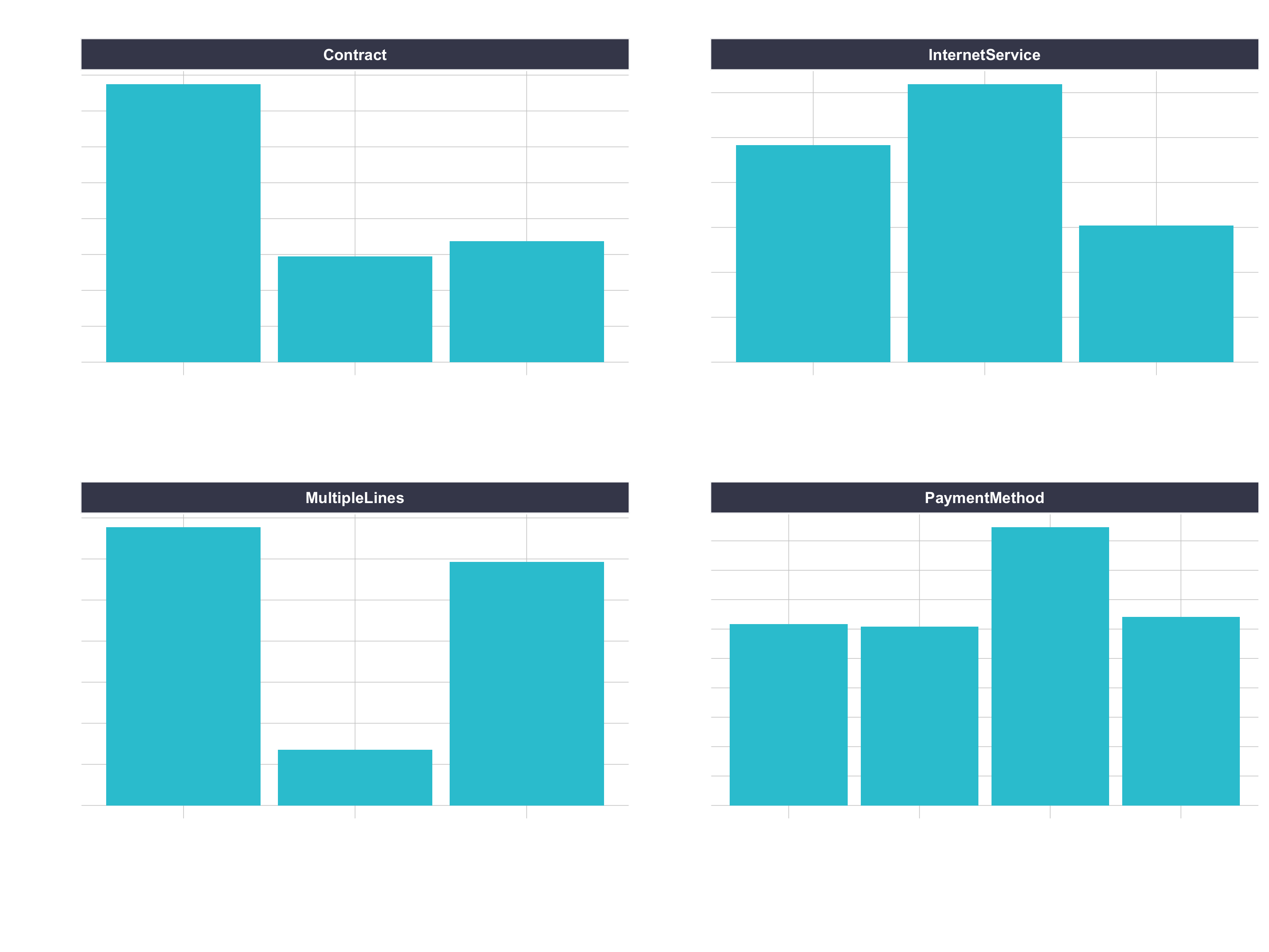
One-hot encoding is the process of converting categorical data to sparse data, which has columns of only zeros and ones (this is also called creating “dummy variables” or a “design matrix”). All non-numeric data will need to be converted to dummy variables. This is simple for binary Yes/No data because we can simply convert to 1’s and 0’s. It becomes slightly more complicated with multiple categories, which requires creating new columns of 1’s and 0`s for each category (actually one less). We have four features that are multi-category: Contract, Internet Service, Multiple Lines, and Payment Method.
churn_data_tbl %>%
        pivot_longer(cols      = c(Contract, InternetService, MultipleLines, PaymentMethod),
                     names_to  = "feature",
                     values_to = "category") %>%
        ggplot(aes(category)) +
          geom_bar(fill = "#2DC6D6") +
          facet_wrap(~ feature, scales = "free") +
          labs(
            title = "Features with multiple categories: Need to be one-hot encoded"
          ) +
          theme(axis.text.x = element_text(angle = 25,
                                           hjust = 1))
Feature Scaling
ANN’s typically perform faster and often times with higher accuracy when the features are scaled and/or normalized (aka centered and scaled, also known as standardizing). Because ANNs use gradient descent, weights tend to update faster. If interested, you can read Sebastian Raschka’s article for a full discussion on the scaling/normalization topic. Tip: When in doubt, standardize the data.
Preprocessing With Recipes
For our model, we use:
- Remove Churn (will be added sperataley to keras)
- Cut the continuous variable for “tenure” to group customers into cohorts.
- Log transform “TotalCharges”.
- One-hot encode the categorical data.
- Mean-center the data.
- Scale the data.
# Create recipe
rec_obj <- recipe( ... , ... ) %>%
    ... %>%
    ... %>%
    ... %>%
    ... %>%
    ... %>%
    ... %>%
    prep( ... )
Solution:
rec_obj <- recipe(Churn ~ ., data = train_tbl) %>%
    step_rm(Churn) %>%
    step_discretize(tenure, options = list(cuts = 6)) %>%
    step_log(TotalCharges) %>%
    step_dummy(all_nominal(), -all_outcomes(), one_hot = T) %>%
    step_center(all_predictors(), -all_outcomes()) %>%
    step_scale(all_predictors(), -all_outcomes()) %>%
    prep(data = train_tbl)
Baking with your recipe:
# Predictors
x_train_tbl <- bake( ... , ... )
x_test_tbl  <- bake( ... , ... )
Now the target. We need to store the actual values (truth) as y_train_vec and y_test_vec, which are needed for modeling our ANN. We convert to a series of numeric ones and zeros which can be accepted by the Keras ANN modeling functions.
# Response variables for training and testing sets
y_train_vec <- ifelse( ... )
y_test_vec  <- ifelse( ... )
Let’s Build our Keras MLP-flavored ANN model. We’ll apply units = 16, which is the number of nodes. We’ll select kernel_initializer = “uniform” and activation = “relu” for both layers. The first layer needs to have the input_shape = 35, which is the number of columns in the training set. We use the layer_dropout() function to drop out layers with rate = 0.10 to remove weights below 10%. We set the kernel_initializer = “uniform” and the activation = “sigmoid” (common for binary classification).
# Building our Artificial Neural Network
model_keras <- keras_model_sequential()

model_keras %>%
    # First hidden layer
    layer_dense(
        units              = 16,
        kernel_initializer = "uniform",
        activation         = "relu",
        input_shape        = ncol(x_train_tbl)) %>%
    # Dropout to prevent overfitting
    layer_dropout(rate = 0.1) %>%
    # Second hidden layer
    layer_dense(
        units              = 16,
        kernel_initializer = "uniform",
        activation         = "relu") %>%
    # Dropout to prevent overfitting
    layer_dropout(rate = 0.1) %>%
    # Output layer
    layer_dense(
        units              = 1,
        kernel_initializer = "uniform",
        activation         = "sigmoid") %>%
    # Compile ANN
    compile(
        optimizer = 'adam',
        loss      = 'binary_crossentropy',
        metrics   = c('accuracy')
    )
model_keras
Let’s use the fit() function to run the ANN on our training data.
You can use the following values:
- batch_size = 50 (number samples per gradient update within each epoch)
- epochs = 35 (number training cycles)
- validation_split = 0.3 (include 30% of the data for model validation, which prevents overfitting)
Remember that the training data has to be in a matrix format
# Fit the keras model to the training data
fit_keras <- fit(
    ...              = ... ,
    ...              = ... ,
    ...              = ... ,
    ...              = ... ,
    ...              = ... ,
    ...              = ...
    )
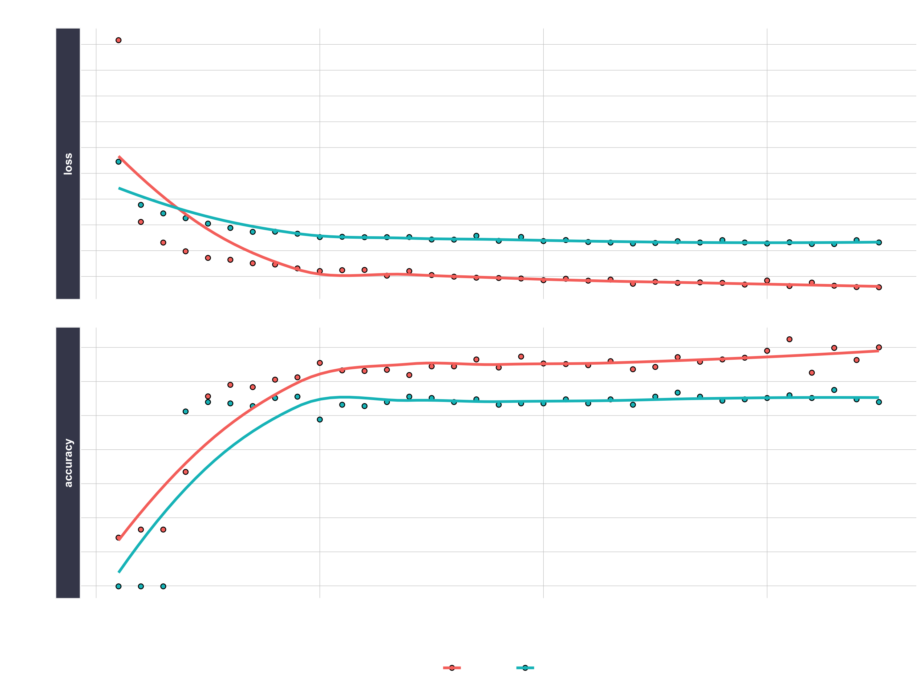
We can inspect the final model. We want to make sure there is minimal difference between the validation accuracy and the training accuracy.
fit_keras
# Plot the training/validation history of our Keras model
plot(fit_keras) +
  labs(title = "Deep Learning Training Results") +
  theme(legend.position  = "bottom",
        strip.placement  = "inside",
        strip.background = element_rect(fill = "#grey"))
Making predictions
We’ve got a good model based on the validation accuracy. Now let’s make some predictions from our keras model on the test data set, which was unseen during modeling (we use this for the true performance assessment). We have two functions to generate predictions:
predict_classes: Generates class values as a matrix of ones and zeros. Since we are dealing with binary classification, we’ll convert the output to a vector.predict_proba: Generates the class probabilities as a numeric matrix indicating the probability of being a class. Again, we convert to a numeric vector because there is only one column output.
# Predicted Class
yhat_keras_class_vec <- predict_classes(object = model_keras, x = as.matrix(x_test_tbl)) %>%
    as.vector()

# Predicted Class Probability
yhat_keras_prob_vec  <- predict_proba(object = model_keras, x = as.matrix(x_test_tbl)) %>%
    as.vector()
Inspect Performance With Yardstick
First, let’s get the data formatted for yardstick. We create a data frame with the truth (actual values as factors), estimate (predicted values as factors), and the class probability (probability of yes as numeric). We use the fct_recode() function from the forcats package to assist with recoding as Yes/No values.
# Format test data and predictions for yardstick metrics
estimates_keras_tbl <- tibble(
    truth      = ... %>% ...,
    estimate   = ... %>% ...,
    class_prob = ...
)

estimates_keras_tbl
## # A tibble: 1,406 x 3
##    truth estimate class_prob
##    <fct> <fct>         <dbl>
##  1 no    yes          0.709
##  2 no    no           0.0277
##  3 yes   yes          0.712
##  4 no    no           0.0286
##  5 no    no           0.0807
##  6 yes   no           0.211
##  7 no    no           0.0913
##  8 yes   no           0.251
##  9 yes   yes          0.735
## 10 no    no           0.302
## # … with 1,396 more rows
Solution:
estimates_keras_tbl <- tibble(
    truth      = as.factor(y_test_vec) %>% fct_recode(yes = "1", no = "0"),
    estimate   = as.factor(yhat_keras_class_vec) %>% fct_recode(yes = "1", no = "0"),
    class_prob = yhat_keras_prob_vec
)
Now that we have the data formatted, we can take advantage of the yardstick package. Confusion Table
We see that the model was by no means perfect, but it did a decent job of identifying customers likely to churn.
# Confusion Table
... %>% ...
##           Truth
## Prediction  no yes
##        no  902 186
##        yes 113 205
Accuracy
We are getting roughly 82% accuracy.
# Accuracy
... %>% ...
## # A tibble: 2 x 3
##   .metric  .estimator .estimate
##   <chr>    <chr>          <dbl>
## 1 accuracy binary         0.796
## 2 kap      binary         0.461
AUC
We can also get the ROC Area Under the Curve (AUC) measurement. AUC is often a good metric used to compare different classifiers and to compare to randomly guessing (AUC_random = 0.50). We need to set the argument event_level to “second”, because the default is to classify 0 as the positive class instead of 1. Our model has AUC = 0.84, which is much better than randomly guessing. Tuning and testing different classification algorithms may yield even better results.
# AUC
... %>% ...
## # A tibble: 1 x 3
##   .metric .estimator .estimate
##   <chr>   <chr>          <dbl>
## 1 roc_auc binary         0.842
Precision And Recall
Precision is when the model predicts “yes”, how often is it actually “yes”. Recall (also true positive rate or specificity) is when the actual value is “yes” how often is the model correct.
# Precision
tibble(
    precision = ...,
    recall    = ...
)
## # A tibble: 1 x 2
##   precision$.metric $.estimator $.estimate recall$.metric $.estimator $.estimate
##   <chr>             <chr>            <dbl> <chr>          <chr>            <dbl>
## 1 precision         binary           0.645 recall         binary           0.524
Precision and recall are very important to the business case: The organization is concerned with balancing the cost of targeting and retaining customers at risk of leaving with the cost of inadvertently targeting customers that are not planning to leave (and potentially decreasing revenue from this group). The threshold above which to predict Churn = “Yes” can be adjusted to optimize for the business problem. This becomes an Customer Lifetime Value optimization problem.
# F1-Statistic
estimates_keras_tbl %>% f_meas(truth, estimate, beta = 1)
## # A tibble: 1 x 3
##   .metric .estimator .estimate
##   <chr>   <chr>          <dbl>
## 1 f_meas  binary         0.578
Explain the model with LIME
LIME stands for Local Interpretable Model-agnostic Explanations, and is a method for explaining black-box machine learning model classifiers. One thing to note is that it’s not setup out-of-the-box to work with keras. The good news is with a few functions we can get everything working properly. We’ll need to make two custom functions:
model_type: Used to tell lime what type of model we are dealing with. It could be classification, regression, survival, etc.predict_model: Used to allow lime to perform predictions that its algorithm can interpret.
The first thing we need to do is identify the class of our model object. We do this with the class() function.
class(model_keras)
## [1] "keras.engine.sequential.Sequential"                         "keras.engine.functional.Functional"
## [3] "keras.engine.training.Model"                                "keras.engine.base_layer.Layer"
## [5] "tensorflow.python.module.module.Module"                     "tensorflow.python.training.tracking.tracking.AutoTrackable"
## [7] "tensorflow.python.training.tracking.base.Trackable"         "keras.utils.version_utils.LayerVersionSelector"
## [9] "keras.utils.version_utils.ModelVersionSelector"             "python.builtin.object"
Next we create our model_type() function. It’s only input is x the keras model. The function simply returns “classification”, which tells LIME we are classifying. It must be named model_type + the first entry of class(model_keras).
# Setup lime::model_type() function for keras
model_type.keras.engine.sequential.Sequential  <- function(x, ...) {
    return("classification")
}
Now we can create our predict_model() function, which wraps keras::predict_proba(). The trick here is to realize that it’s inputs must be x a model, newdata a dataframe object (this is important), and type which is not used but can be use to switch the output type. The output is also a little tricky because it must be in the format of probabilities by classification:
# Setup lime::predict_model() function for keras
predict_model.keras.engine.sequential.Sequential <- function(x, newdata, type, ...) {
    pred <- predict_proba(object = x, x = as.matrix(newdata))
    return(data.frame(Yes = pred, No = 1 - pred))
}
Run this next script to show you what the output looks like and to test our predict_model() function. See how it’s the probabilities by classification. It must be in this form for model_type = "classification".
library(lime)
# Test our predict_model() function
predict_model(x = model_keras, newdata = x_test_tbl, type = 'raw') %>%
    tibble::as_tibble()
## # A tibble: 1,406 x 2
##       Yes    No
##     <dbl> <dbl>
##  1 0.673  0.327
##  2 0.0504 0.950
##  3 0.745  0.255
##  4 0.0412 0.959
##  5 0.0519 0.948
##  6 0.299  0.701
##  7 0.0957 0.904
##  8 0.203  0.797
##  9 0.687  0.313
## 10 0.263  0.737
## # … with 1,396 more rows
Now we can create an explainer using the lime() function. Just pass the training data. You can set bin_continuous = FALSE. We could tell the algorithm to bin continuous variables, but this may not make sense for categorical numeric data that we didn’t change to factors.
# Run lime() on training set
explainer <- lime::lime(
    ...            = ...,
    ...            = ... ,
    bin_continuous = FALSE)
Now we run the explain() function, which returns our explanation. This can take a minute to run so we limit it to just the first ten rows of the test data set.
explanation <- lime::explain(
    x_test_tbl[1:10,],
    ...    = ...,
    ...    = ...,
    ...    = ...,
    ...    = ...)
The payoff for the work we put in using LIME are the feature importance plots. Create the plots with plot_features() and plot_explanations(). One thing we need to be careful with the LIME visualization is that we are only doing a sample of the data, in our case the first 10 test observations. Therefore, we are gaining a very localized understanding of how the ANN works. However, we also want to know on from a global perspective what drives feature importance.
We can perform a correlation analysis on the training set as well to help glean what features correlate globally to “Churn”. We’ll use the corrr package, which performs tidy correlations with the function correlate(). We can get the correlations as follows.
# Feature correlations to Churn
corrr_analysis <- x_train_tbl %>%
    mutate(Churn = y_train_vec) %>%
    correlate() %>%
    focus(Churn) %>%
    rename(feature = rowname) %>%
    arrange(abs(Churn)) %>%
    mutate(feature = as_factor(feature))
corrr_analysis
The correlation visualization helps in distinguishing which features are relavant to Churn.
# Correlation visualization
corrr_analysis %>%
  ggplot(aes(x = ..., y = fct_reorder(..., desc(...)))) +
  geom_point() +

  # Positive Correlations - Contribute to churn
  geom_segment(aes(xend = ..., yend = ...),
               color = "red",
               data = corrr_analysis %>% filter(... > ...)) +
  geom_point(color = "red",
             data = corrr_analysis %>% filter(... > ...)) +

  # Negative Correlations - Prevent churn
  geom_segment(aes(xend = 0, yend = feature),
               color = "#2DC6D6",
               data = ... +
  geom_point(color = "#2DC6D6",
             data = ... +

  # Vertical lines
  geom_vline(xintercept = 0, color = "#f1fa8c", size = 1, linetype = 2) +
  geom_vline( ... ) +
  geom_vline( ... ) +

  # Aesthetics
  labs( ... )
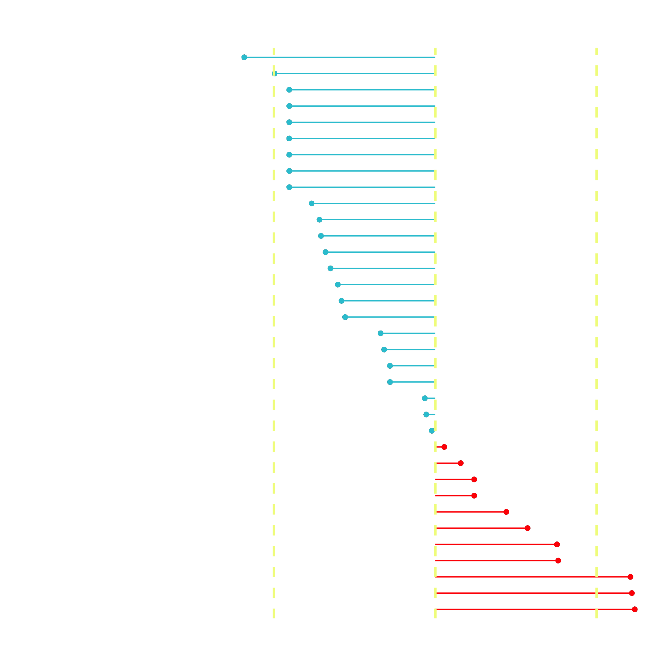
The correlation analysis helps us quickly disseminate which features that the LIME analysis may be excluding. We can see that the following features are highly correlated (magnitude > 0.25):
Increases Likelihood of Churn (Red):
- Tenure = Bin 1 (<12 Months)
- Internet Service = “Fiber Optic”
- Payment Method = “Electronic Check”
Decreases Likelihood of Churn (Turquoise):
- Contract = “Two Year”
- Total Charges (Note that this may be a biproduct of additional services such as Online Security)