Supervised ML - Regression (II)
Let’s apply our newly acquired machine learning skills to a business case!
Business case
In this case we are using the scraped data from the bike manufacturer Canyon again. This is an extension of the data that you already know.
At the beginning we need to load the following packages:
# Standard
library(tidyverse)

# Modeling
library(parsnip)

# Preprocessing & Sampling
library(recipes)
library(rsample)

# Modeling Error Metrics
library(yardstick)

# Plotting Decision Trees
library(rpart.plot)
Our goal is to figure out what gaps exist in the products and come up with a pricing algorithm that will help us to determine a price, if we were to come up with products in that product cateogry.
Data preparation
I. Data Exploration
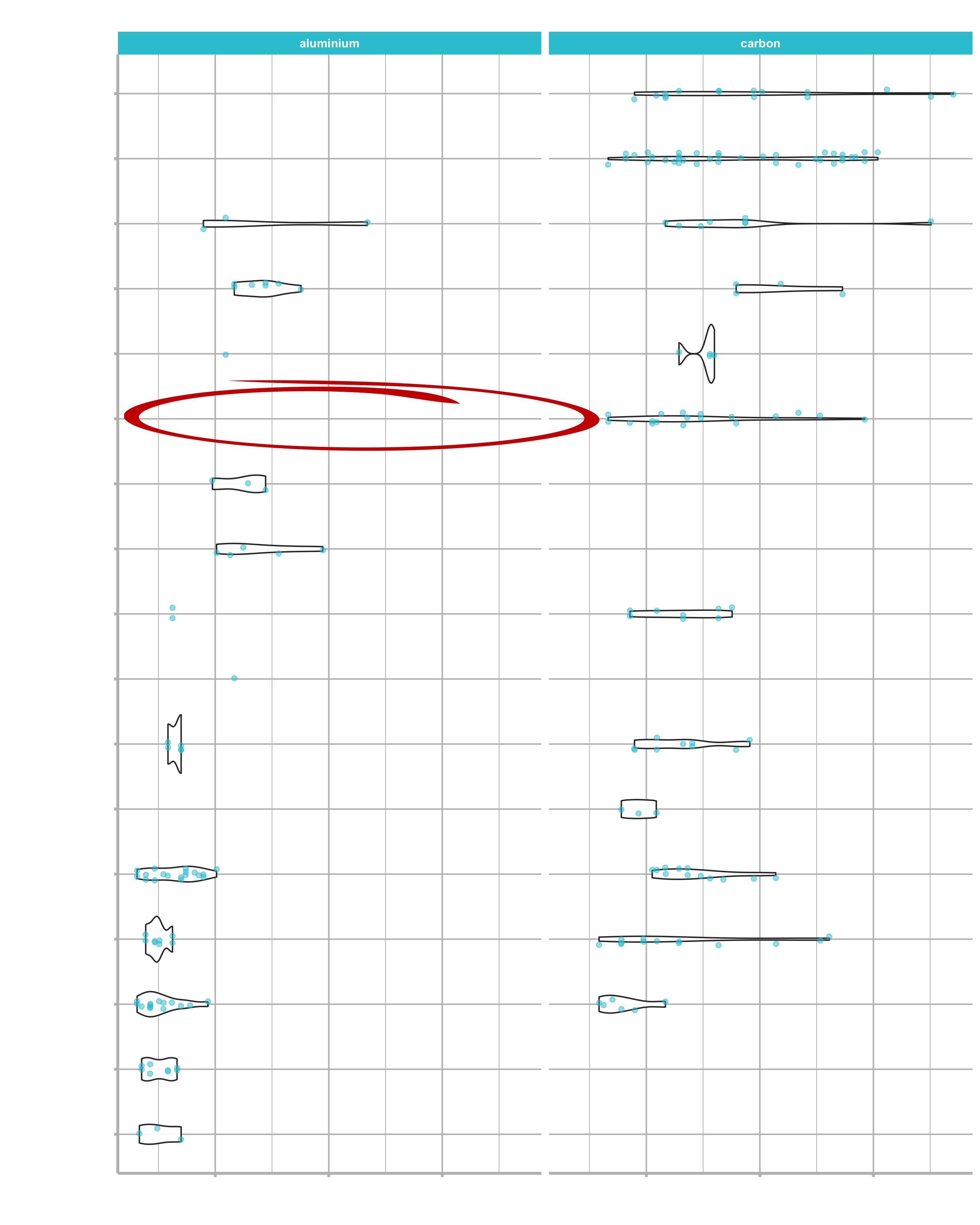
To determine possible product gaps, let’s start with visualizing the data. It would be interesting to see the sales for each category_2 separated by the frame material. Unfortunately, we do not have the sales number. Instead, let’s just use the stock numbers as a proxy.
# Modeling ----------------------------------------------------------------
bike_orderlines_tbl <- readRDS("~/bike_orderlines_tbl.rds")
glimpse(bike_orderlines_tbl)

model_sales_tbl <- bike_orderlines_tbl %>%
    select(total_price, model, category_2, frame_material) %>%

    group_by(model, category_2, frame_material) %>%
    summarise(total_sales = sum(total_price)) %>%
    ungroup() %>%

    arrange(desc(total_sales))

model_sales_tbl %>%
    mutate(category_2 = as_factor(category_2) %>%
               fct_reorder(total_sales, .fun = max) %>%
               fct_rev()) %>%

    ggplot(aes(frame_material, total_sales)) +
    geom_violin() +
    geom_jitter(width = 0.1, alpha = 0.5, color = "#2c3e50") +
    #coord_flip() +
    facet_wrap(~ category_2) +
    scale_y_continuous(labels = scales::dollar_format(scale = 1e-6, suffix = "M", accuracy = 0.1)) +
    tidyquant::theme_tq() +
    labs(
        title = "Total Sales for Each Model",
        x = "Frame Material", y = "Revenue"
    )
Don’t get confused by the image. For this plot, different data was used. But the underlying information is the same.
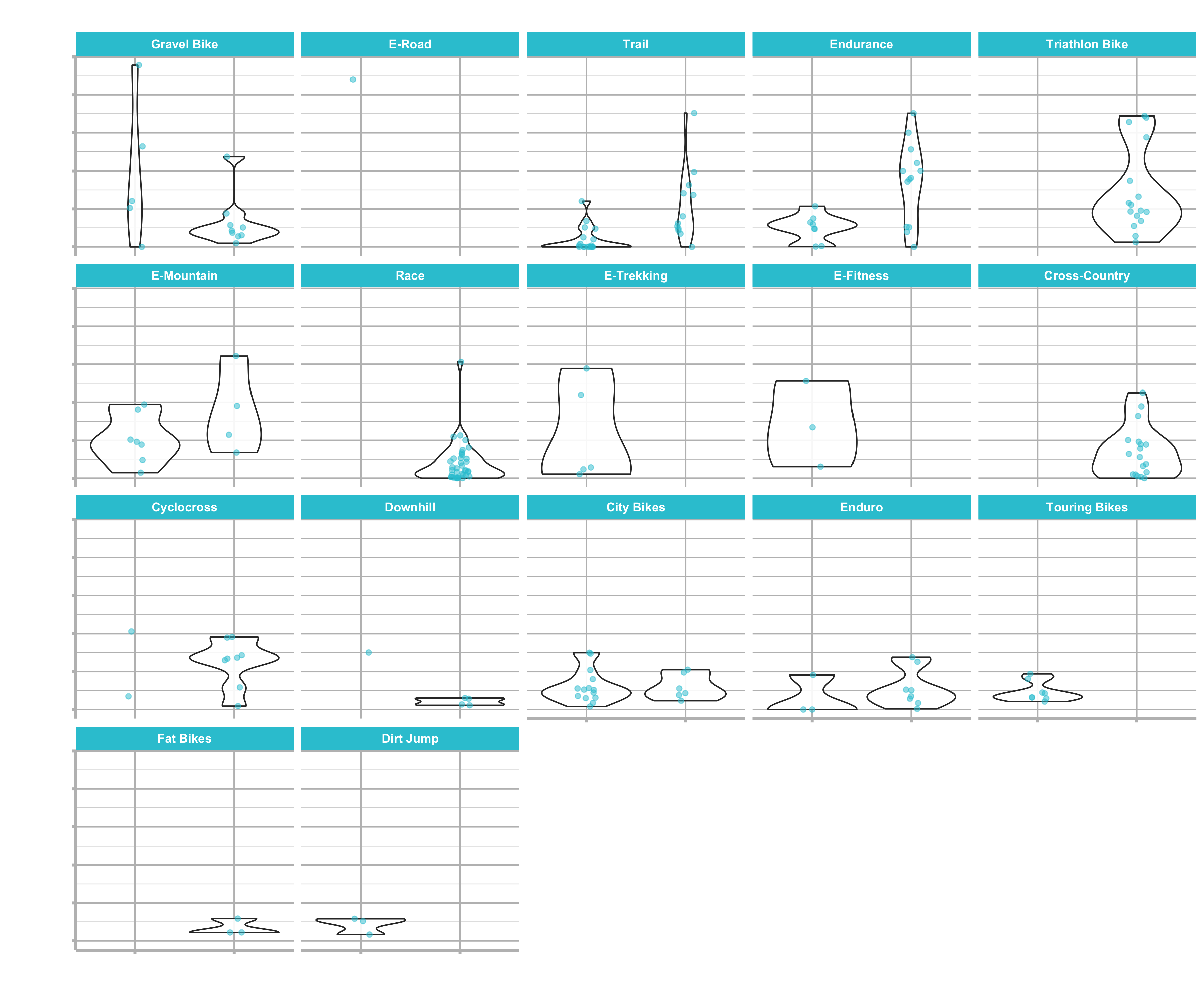
We are showing this vizualisation, because we can use it as a game plan. We want to answer the questions
Problem definition
- Which Bike Categories are in high demand?
- Which Bike Categories are under represented?
Goal
- Use a pricing algorithm to determine a new product price in a category gap
We have the bike models separated into aluminium and carbon frames. The reason for that is splitting the bikes in lower end products (alu) and higher end (carbon) ones.
You can see that most categories offer both specifications and they make a fair amount of the lower end products as well. But not all categories have an aluminium option. Those products with “High-End” (carbon) option only could be missing out on revenues.
We can focus on those product gaps (products like “Cross-Country” and “Fat Bikes”) for new product development. Based on this information, we are going to come up with a pricing algorithm, that allows us to price models and see if it is going to be a profitable venture. We could generate significant revenue by filling in the gaps, if we use the other categories as a benchmark.
II. Data Preparation & Feature Engineering
At first we have to set up our data. To be able to predict bike models, I have gathered the groupsets (so that we have more features than just the weight and the frame material) for each bike model. A bike’s groupset, refers to any mechanical or electronic parts that are involved in braking, changing gear, or the running of the drivetrain. That means the shifters, brake levers, front and rear brake calipers, front and rear derailleurs, crankset, bottom bracket, chain, and cassette.
If you’re buying a bike, then, after the frame, the groupset is the second thing that you should look at, and is a key determining factor in working out whether the bike in front of you offers good value for money or not.
There are three main manufacturers of groupsets and bike components. Shimano is the largest and best known, while the other two of the “big three” are Campagnolo and SRAM. All three manufacturers offer a range of groupsets (divided into road and MTB) at competing price points. Groupsets are arranged into heirarchies, with compatible parts grouped in order of quality and price.
Most components are designed to work best with those in the same brand and hierarchy. Cross-compatibility is not the norm, especially between the three different brands, although there are of course exceptions. That is why I only examine one component (the Rear Derailleur, or if not existent the Shift lever) of the bikes to categorize the them.
The following step creates dummy variables on this non-numeric data by setting flags (0 or 1) for each component. We could have done this with the recipes approach as well step_dummy(all_nominal(), - all_outcomes()).
bike_features_tbl <- readRDS("~/bike_features_tbl.rds")
glimpse(bike_features_tbl)

bike_features_tbl <- bike_features_tbl %>%
    select(model:url, `Rear Derailleur`, `Shift Lever`) %>%
    mutate(
      `shimano dura-ace`        = `Rear Derailleur` %>% str_to_lower() %>% str_detect("shimano dura-ace ") %>% as.numeric(),
      `shimano ultegra`         = `Rear Derailleur` %>% str_to_lower() %>% str_detect("shimano ultegra ") %>% as.numeric(),
      `shimano 105`             = `Rear Derailleur` %>% str_to_lower() %>% str_detect("shimano 105 ") %>% as.numeric(),
      `shimano tiagra`          = `Rear Derailleur` %>% str_to_lower() %>% str_detect("shimano tiagra ") %>% as.numeric(),
      `Shimano sora`            = `Rear Derailleur` %>% str_to_lower() %>% str_detect("shimano sora") %>% as.numeric(),
      `shimano deore`           = `Rear Derailleur` %>% str_to_lower() %>% str_detect("shimano deore(?! xt)") %>% as.numeric(),
      `shimano slx`             = `Rear Derailleur` %>% str_to_lower() %>% str_detect("shimano slx") %>% as.numeric(),
      `shimano grx`             = `Rear Derailleur` %>% str_to_lower() %>% str_detect("shimano grx") %>% as.numeric(),
      `Shimano xt`              = `Rear Derailleur` %>% str_to_lower() %>% str_detect("shimano deore xt |shimano xt ") %>% as.numeric(),
      `Shimano xtr`             = `Rear Derailleur` %>% str_to_lower() %>% str_detect("shimano xtr") %>% as.numeric(),
      `Shimano saint`           = `Rear Derailleur` %>% str_to_lower() %>% str_detect("shimano saint") %>% as.numeric(),
      `SRAM red`                = `Rear Derailleur` %>% str_to_lower() %>% str_detect("sram red") %>% as.numeric(),
      `SRAM force`              = `Rear Derailleur` %>% str_to_lower() %>% str_detect("sram force") %>% as.numeric(),
      `SRAM rival`              = `Rear Derailleur` %>% str_to_lower() %>% str_detect("sram rival") %>% as.numeric(),
      `SRAM apex`               = `Rear Derailleur` %>% str_to_lower() %>% str_detect("sram apex") %>% as.numeric(),
      `SRAM xx1`                = `Rear Derailleur` %>% str_to_lower() %>% str_detect("sram xx1") %>% as.numeric(),
      `SRAM x01`                = `Rear Derailleur` %>% str_to_lower() %>% str_detect("sram x01|sram xo1") %>% as.numeric(),
      `SRAM gx`                 = `Rear Derailleur` %>% str_to_lower() %>% str_detect("sram gx") %>% as.numeric(),
      `SRAM nx`                 = `Rear Derailleur` %>% str_to_lower() %>% str_detect("sram nx") %>% as.numeric(),
      `SRAM sx`                 = `Rear Derailleur` %>% str_to_lower() %>% str_detect("sram sx") %>% as.numeric(),
      `SRAM sx`                 = `Rear Derailleur` %>% str_to_lower() %>% str_detect("sram sx") %>% as.numeric(),
      `Campagnolo potenza`      = `Rear Derailleur` %>% str_to_lower() %>% str_detect("campagnolo potenza") %>% as.numeric(),
      `Campagnolo super record` = `Rear Derailleur` %>% str_to_lower() %>% str_detect("campagnolo super record") %>% as.numeric(),
      `shimano nexus`           = `Shift Lever`     %>% str_to_lower() %>% str_detect("shimano nexus") %>% as.numeric(),
      `shimano alfine`          = `Shift Lever`     %>% str_to_lower() %>% str_detect("shimano alfine") %>% as.numeric()
    ) %>%
  # Remove original columns
  select(-c(`Rear Derailleur`, `Shift Lever`)) %>%
  # Set all NAs to 0
  mutate_if(is.numeric, ~replace(., is.na(.), 0))
Let’s order and tidy the tibble a bit. We need the following data:
- ID: Tells us which rows are being sampled
- Target (price): What we are trying to predict
- Predictors (all other columns): Data that our algorithms will use to build relationships to target
Adding good engineered features is the #1 way to boost model performance.
# 2.0 TRAINING & TEST SETS ----
bike_features_tbl <- bike_features_tbl %>%

  mutate(id = row_number()) %>%

  select(id, everything(), -url)
III. Splitting the Data
Splitting the data into training & test sets helps to prevent overfitting and improve model generalization (the ability of a model to perform well on future data). Even better is cross-validation. This is an advanced concept, which will be shown later.
The initial_split() function returns a split object with training and testing set sets. Let’s use 80 % of the data for the training set and 20 % for the test set. Remember that the strata argument causes the random sampling to be conducted within the stratification variable. It helps to ensure that the number of data points in the analysis data is equivalent to the proportions in the original data set. The category_2 feature has 17 levels. A random split may not have all these levels in the training set, which would be bad. We can prevent this by adding category_2 as the stratification variable.
bike_features_tbl %>% distinct(category_2)

# run both following commands at the same time
set.seed(seed = 1113)
split_obj <- rsample::initial_split(bike_features_tbl, prop   = 0.80,
                                                       strata = "category_2")

# Check if testing contains all category_2 values
split_obj %>% training() %>% distinct(category_2)
split_obj %>% testing() %>% distinct(category_2)

# Assign training and test data
train_tbl <- training(split_obj)
test_tbl  <- testing(split_obj)

# We have to remove spaces and dashes from the column names
train_tbl <- train_tbl %>% set_names(str_replace_all(names(train_tbl), " |-", "_"))
test_tbl  <- test_tbl  %>% set_names(str_replace_all(names(test_tbl),  " |-", "_"))
1. Linear Regression
Linear regression is the first modeling algorithm, which we will implement. It’s the simplest method to understand and it’s the basis for more complex algorithms like the Elastic Net (coming soon).
Fitting a line to data
This covers the concept of ordinary least squares regression, which uses a straight line to minimize the sum of the squared residuals (difference between prediction and actual values that gets squared to remove any negatives).
Linear Regression
Once you understand the concept of fitting a line to data, Linear Regression takes the concept and applies it to modeling.
Multiple Linear Regression
Multiple linear regression is just an extension of linear regression with many predictors
Take a look at the
modellist and filter for the parsnip package to find possible model types and engines. For now, we are focusing on
linear_reg() and two different engines (the underlying models that are used with parsnip). First, we start with a simple linear regression with the lm engine, that comes with base R and then we will try to improve the model using the glmnet algorithm.
1.1 Linear Regression (simple) - Model 1
1.1.1 Model
The parsnip::linear_reg() function creates a parsnip specification for a linear regression.
Take a look at the following documentation: ?linear_reg
At the top you can see the model parameters (main parameters for underlying model are controlled here: penalty and mixture). Because linear regression does not have any adjustable parameters, we don’t have to worry about those tunable values yet.
Each model is built with three steps (with the Parsnip API):
- Create a model:
linear_reg() - Set an engine:
set_engine() - Fit the model to data:
fit()
Let’s use for the first model only category_2 and frame_material as variables.
# 3.0 LINEAR METHODS ----
# 3.1 LINEAR REGRESSION - NO ENGINEERED FEATURES ----

# 3.1.1 Model ----
?lm # from the stats package
?set_engine
?fit # then click Estimate model parameters and then fit at the bottom

model_01_linear_lm_simple <- linear_reg(mode = "regression") %>%
    set_engine("lm") %>%
    fit(price ~ category_2 + frame_material, data = train_tbl)
Make predictions using a parsnip model_fit object.
?predict.model_fit

model_01_linear_lm_simple %>%
    predict(new_data = test_tbl)
## # A tibble: 42 x 1
##    .pred
##    <dbl>
## 1 4678.
## 2 3280.
## 3 3370.
## 4 3618.
## 5 3618.
## 6 4678.
## 7 4678.
## 8 4678.
## 9 4678.
## 10 4678.
## # … with 35 more rows
We calculate model metrics comparing the test data predictions with the actual values to get a baseline model performance. MAE and RMSE are important concepts:
- Residuals: Difference between actual (truth) and prediction (estimate from the model)
- MAE (Mean absolute error): Absolute value of residuals generates the magnitude of error. Take the average to get the average error.
- RMSE (Root mean squared error): Square the residuals to remove negative sign. Take the average. Take the square root of average to return to units of initial error term.
yardstick::metrics() calculates the common metrics comparing a “truth” (price) to an “estimate” (.pred).
?metrics

model_01_linear_lm_simple %>%
    predict(new_data = test_tbl) %>%

    bind_cols(test_tbl %>% select(price)) %>%

    # Manual approach
    # mutate(residuals = price - .pred) %>%
    #
    # summarize(
    #   mae  = abs(residuals) %>% mean(),
    #   rmse = mean(residuals^2)^0.5
    # )

    yardstick::metrics(truth = price, estimate = .pred)
Model Interpretability for Linear Models - How it works
Linear models are amazingly easy to interpret (provided we understand how a linear modeling equation works). The prediction function looks like this:
Where the:
- Intercept: Is what all predictions start out at (e.g. 1142 €)
- Model Coefficients (c1 through cN): Estimates that adjust the features weight in the model
- Features (1 through N): The value of the Feature in the model (categorical are encoded as binary, numeric are left as numeric)
How do we make this interpretable?
One of the huge advantages of linear regression is that it is very explainable. This is very critical to helping communicate models to stakeholders as you want to be able to tell them what each feature is doing within that model.
Making a Linear Regression interpretable is very easy provided all of the predictors are categorical (meaning any numeric predictors need to be binned so their values are interpreted in the model as low/med/high). The categorical nature is necessary so we can create a plot like this:
In the plot, each predictor has a coefficient that is in terms of the final output (i.e. price of the bike model). For a carbon Gravel Bike the linear equation becomes:
Everything else in the model is zero because the features are not present.
We can then interpret the model by adding the coefficients.
Where each of the coefficients are in terms of the final output (e.g. euros) because all of the Features are essentially binary (e.g. is the Bike Model Configuration == Carbon? yes or no?).
Dealing with numeric predictors
For numeric features, we just need to bin them prior to performing the regression to make them categorical in bins like High, Medium, Low. Otherwise, the coefficients will be in the wrong scale for the numeric predictors. We have discuessed already how to do this - You have a few options, and my preference is using a mutate() with case_when(). You can find the price at the 33th and 66th quantile with quantile(probs = c(0.33, 0.66)). Then just use those values to create low, medium, high categories.
Our models in this session have categorical data, but in the future just remember that numeric predictors will need to be converted to categorical (i.e. binned) prior to making an interpretable plot like the one above.
1.1.2 Model Explanation
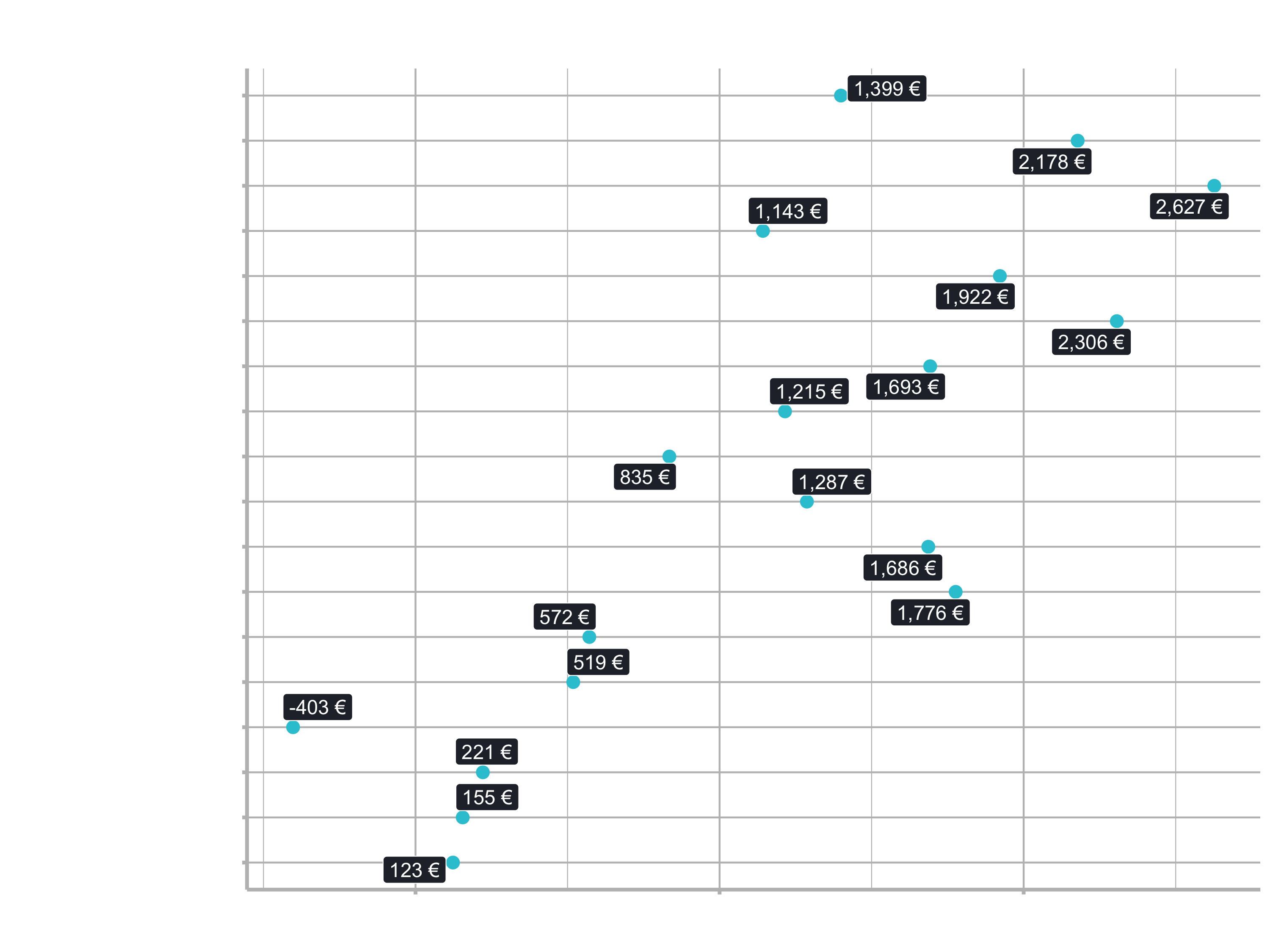
The model data from the stats::lm() function is stored in the “fit” element, which we can easily plot. To arrange the importance, we can arrange the data by the p-value. Generally speaking: the lower the p-value, the more important is the term to the linear regression model.
# 3.1.2 Feature Importance ----
View(model_01_linear_lm_simple) # You will see the coefficients in the element "fit"

# tidy() function is applicable for objects with class "lm"
model_01_linear_lm_simple$fit %>% class()

model_01_linear_lm_simple$fit %>%
  broom::tidy() %>%
  arrange(p.value) %>%
  mutate(term = as_factor(term) %>% fct_rev()) %>%

  ggplot(aes(x = estimate, y = term)) +
  geom_point(color = "#2dc6d6", size = 3) +
  ggrepel::geom_label_repel(aes(label = scales::dollar(estimate, accuracy = 1, suffix = " €", prefix = "")),
                            size = 4, fill = "#272A36", color = "white") +
  scale_x_continuous(labels = scales::dollar_format(suffix = " €", prefix = "")) +
  labs(title = "Linear Regression: Feature Importance",
       subtitle = "Model 01: Simple lm Model")
Metrics helper
Before we are going to the next model, let’s create a helper function, because calculating the metrics will be quite repetitive.
# 3.1.3 Function to Calculate Metrics ----

# Code we used earlier
model_01_linear_lm_simple %>%
    predict(new_data = test_tbl) %>%

    bind_cols(test_tbl %>% select(price)) %>%
    yardstick::metrics(truth = price, estimate = .pred)

# Generalized into a function
calc_metrics <- function(model, new_data = test_tbl) {

    model %>%
        predict(new_data = new_data) %>%

        bind_cols(new_data %>% select(price)) %>%
        yardstick::metrics(truth = price, estimate = .pred)

}

model_01_linear_lm_simple %>% calc_metrics(test_tbl)
## # A tibble: 3 x 3
##   .metric .estimator .estimate
##   <chr>   <chr>          <dbl>
## 1 rmse    standard    1369.
## 2 rsq     standard       0.414
## 3 mae     standard    924.
1.2 Linear regression (complex) - Model 2
1.2.1 Model
Next, we want to show the impact of adding in some engineered features. This is going to be a good example, because it shows how we can quickly improve the model, without even changing the modeling algorithm, but actually adding in better features to do the modeling on. Feature engineering is a general term for creating features that add to the predictiveness of the model. Many times this requires domain knowledge.
price ~ . tells parsnip to fit a model to price as a function of all the predictor columns
# 3.2 LINEAR REGRESSION - WITH ENGINEERED FEATURES ----

# 3.2.1 Model ----
model_02_linear_lm_complex <- linear_reg("regression") %>%
    set_engine("lm") %>%

    # This is going to be different. Remove unnecessary columns.
    fit(price ~ ., data = train_tbl %>% select(-c(id:weight), -category_1, -c(category_3:gender)))

model_02_linear_lm_complex %>% calc_metrics(new_data = test_tbl)
## # A tibble: 3 x 3
##   .metric .estimator .estimate
##   <chr>   <chr>          <dbl>
## 1 rmse    standard    971.
## 2 rsq     standard       0.712
## 3 mae     standard     801.
The MAE dropped quite a bit. We have an improvement of over 100 € in our ability to correctly predict these bikes and we didn’t even change our model.
1.2.2 Model Explanation
# 3.2.2 Feature importance ----
model_02_linear_lm_complex$fit %>%
  broom::tidy() %>%
  arrange(p.value) %>%
  mutate(term = as_factor(term) %>% fct_rev()) %>%

  ggplot(aes(x = estimate, y = term)) +
  geom_point(color = "#2dc6d6", size = 3) +
  ggrepel::geom_label_repel(aes(label = scales::dollar(estimate, accuracy = 1, suffix = " €", prefix = "")),
                            size = 4, fill = "#272A36", color = "white") +
  scale_x_continuous(labels = scales::dollar_format(suffix = " €", prefix = "")) +
  labs(title = "Linear Regression: Feature Importance",
       subtitle = "Model 02: Complex lm Model")
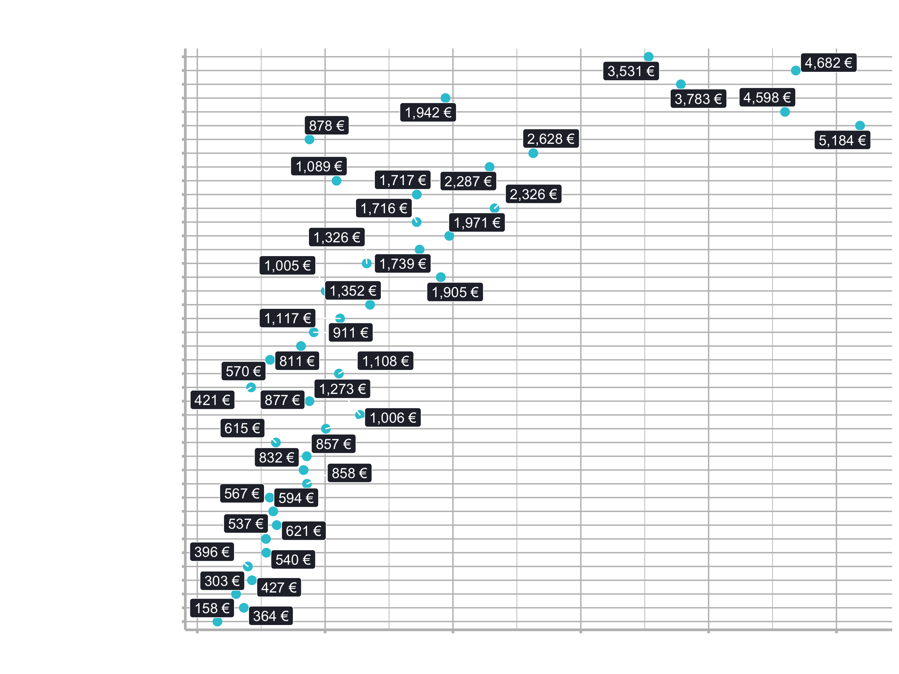
There is no feature for Aluminium Frame or for City Bikes. By default, the models begin with the 1st alphabetical element in the category:
- Default frame material: Aluminium
- Default category_2: City Bikes
2. GLM Regularized Regression
The first machine learning technique we will implement is the Elastic Net - A high performance linear method that uses a combination of L1 and L2 regularization to penalize columns that have low predictive utility. What does this mean?
These videos from StatQuest will help you get up to speed on key concepts including Regularization, Ridge Regression, LASSO Regression, and Elastic Net.
Regularization Part 1 - Ridge Regression
L2 Regularization comes from Ridge Regression.
Regularization Part 2 - LASSO Regression
L1 Regularization comes from LASSO Regression
Regularization Part 3 - Elastic Net Regression
Combines L1 and L2 Regularization into one modeling algorithm
2.1 GLM Regularized Regression (Model 03): GLMNET (Elastic Net)
2.1.1 Model
Regularization: A penalty factor that is applied to columns that are present but that have lower predicitive value.
?linear_reg
?glmnet::glmnet
It is very similiar to the standard linear regression, but now we can use the arguments penalty and mixture.
# 3.3 PENALIZED REGRESSION ----

# 3.3.1 Model ----
?linear_reg
?glmnet::glmnet

model_03_linear_glmnet <- linear_reg(mode    = "regression",
                                     penalty = 10,
                                     mixture = 0.1) %>%
    set_engine("glmnet") %>%
    fit(price ~ ., data = train_tbl %>% select(-c(id:weight), -category_1, -c(category_3:gender)))

model_03_linear_glmnet %>% calc_metrics(test_tbl)
## # A tibble: 3 x 3
##   .metric .estimator .estimate
##   <chr>   <chr>          <dbl>
## 1 rmse    standard    953.
## 2 rsq     standard       0.728
## 3 mae     standard     788.
Unfortunately it did improve the model just slightly. Try tuning yourself. See if you can improve further. Play around with the penalty and the mixture arguments and check the MAE value. There are several different combinations. Systematically adjusting the model parameters to optimize the performance is called Hyper Parameter Tuning. Grid Search, which we have mentioned earlier, is a popular hyperparameter tuning method of producing a “grid”, that has many combinations of parameters. Hyper Parameter Tuning, Grid Search & Cross Validation: All of these advanced topics are covered in detail in the next sessions.
2.1.2 Model Explanation
# 3.3.2 Feature Importance ----
model_03_linear_glmnet$fit %>%
    broom::tidy() %>%
    filter(lambda >= 10 & lambda < 11) %>%

    # No p value here
    arrange(desc(abs(estimate))) %>%
    mutate(term = as_factor(term) %>% fct_rev()) %>%

    ggplot(aes(x = estimate, y = term)) +
    geom_point() +
    ggrepel::geom_label_repel(aes(label = scales::dollar(estimate, accuracy = 1)),
                              size = 3) +
    scale_x_continuous(labels = scales::dollar_format()) +
    labs(title = "Linear Regression: Feature Importance",
         subtitle = "Model 03: GLMNET Model")
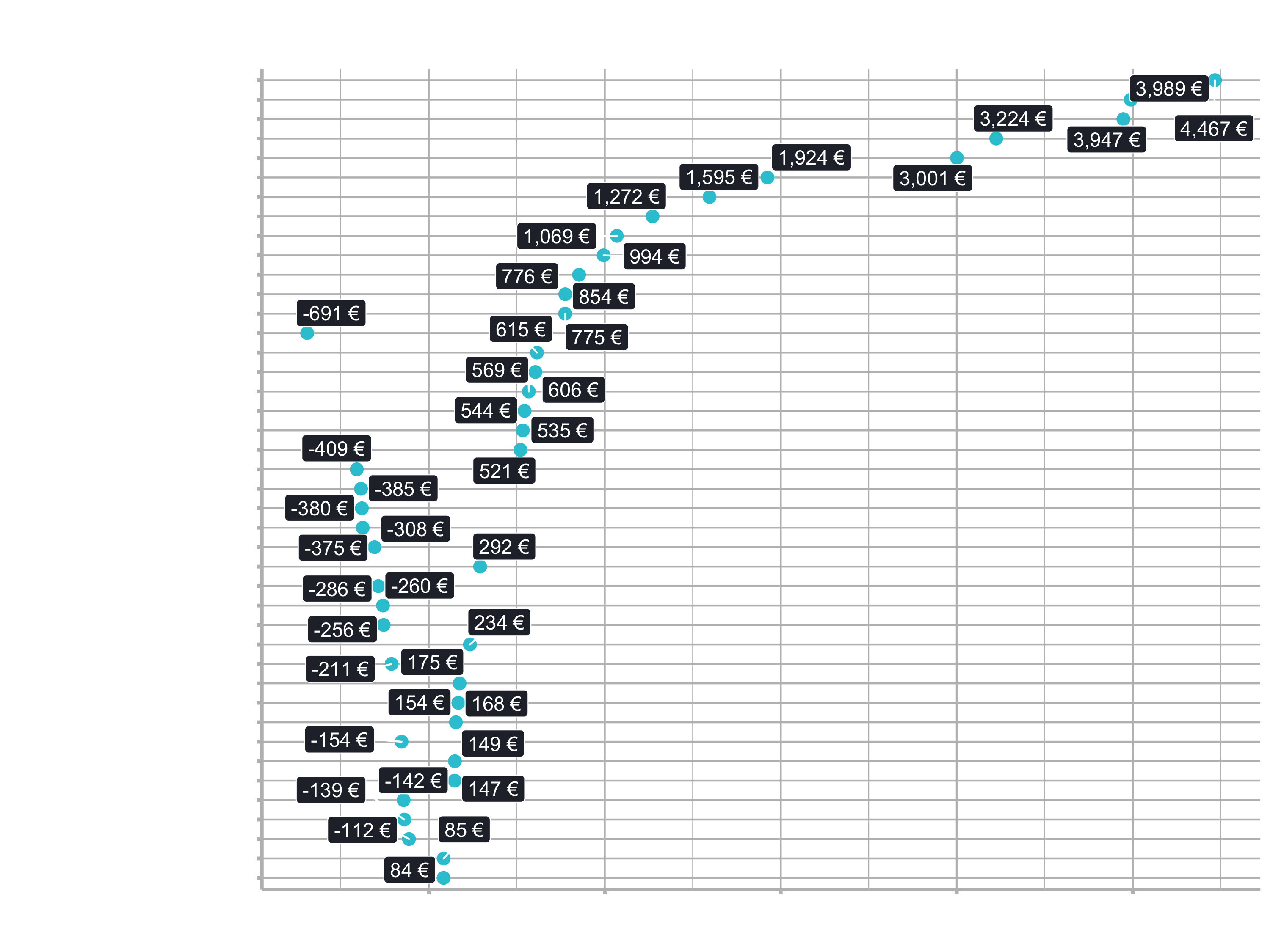
You can see, the model has a lot more magnitude on the top features meaning the less important features get much more penalized. It is possible to get a better model weighing features more or less. But since all features are pretty much related, we got no big difference.
3. Tree-Based Methods
Pro:
- High performance
- Naturally incorporate Non-Linear relationships & interactions
- Minimal preprocessing
Con:
- Less Explainability
Decision trees are very explainable, but as soon as you get to Random Forest & XGBoost they become less explainable (that’s way they are called “Black-Box” models)
3.1 Decision Trees - Model 4
Our journey into tree-based models begins with Decision Trees, which are the basis for more complex methods (higher performance) such as Random Forest and Gradient Boosted Machines (GBMs). The following StatQuest video provides an excellent overview of how Decision Trees work.
3.1.1 Model
?decision_tree
These are our arguments:
- cost_complexity
- tree_depth
- min_n
Avoid Overfitting: Tree-Based methods can become over-fit if we let the nodes contain too few data points or the trees to grow too large (high variance) Avoid Underfitting: If tree is too shallow or too many data points are required per node, tree becomes under-fit (high bias)
We have to tune these parameters above to come up with the best possible decision tree. We are going to use the engine for rpart:
?rpart::rpart
# 4.0 TREE-BASED METHODS ----
# 4.1 DECISION TREES ----
# 4.1.1 Model ----

model_04_tree_decision_tree <- decision_tree(mode = "regression",

              # Set the values accordingly to get started
              cost_complexity = 0.001,
              tree_depth      = 5,
              min_n           = 7) %>%

    set_engine("rpart") %>%
    fit(price ~ ., data = train_tbl %>% select(-c(id:weight), -category_1, -c(category_3:gender)))

model_04_tree_decision_tree %>% calc_metrics(test_tbl)
## # A tibble: 3 x 3
##   .metric .estimator .estimate
##   <chr>   <chr>          <dbl>
## 1 rmse    standard    1165.
## 2 rsq     standard       0.617
## 3 mae     standard     976.
Min N = 20 results in underfitting Min N = 3 results in overfitting Min N = 7 is just right
3.1.2 Model Explanation
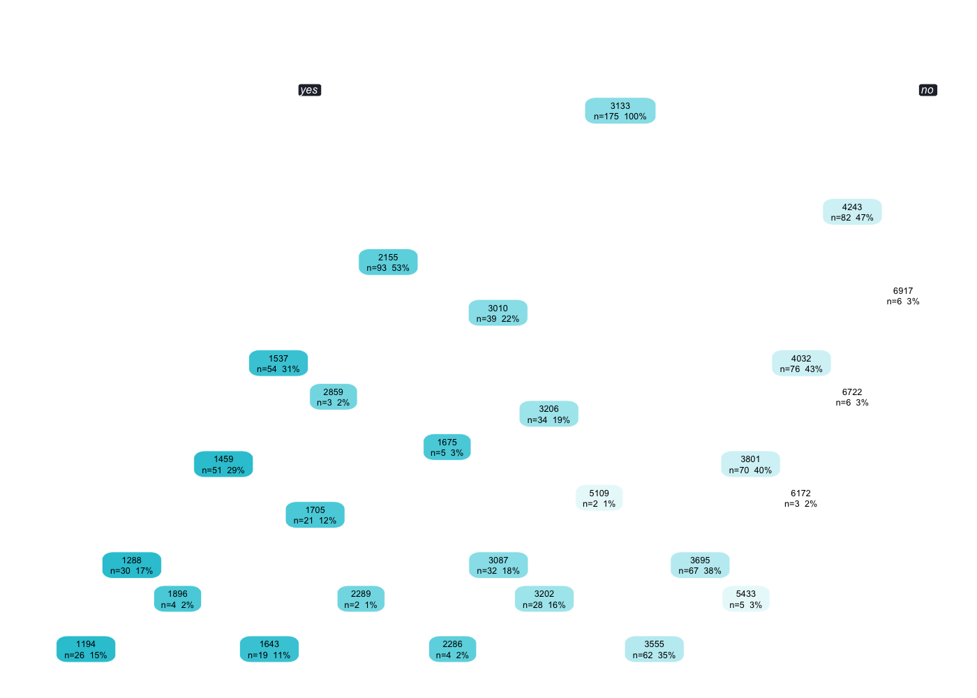
Let’s use rpart.plot() to plot our tree. There are many arguments, that you can adjust.
# 4.1.2 Decision Tree Plot ----
?rpart.plot()

model_04_tree_decision_tree$fit %>%
    rpart.plot(roundint = FALSE)

# Optimze plot
model_04_tree_decision_tree$fit %>%
    rpart.plot(
        roundint = FALSE,
        type = 1,
        extra = 101, # see help page
        fallen.leaves = FALSE, # changes the angles from 90 to 45-degree
        cex = 0.8, # font size
        main = "Model 04: Decision Tree", # Adds title
        box.palette = "Blues"
        )

show.prp.palettes()
3.2 Random Forest
The Random Forest is a critical machine learning tool in your arsenal as a data scientist (along with the GLM that you’ve seen previously). The StatQuest video below examines how the Random Forest generates high-performance via the boostrapped resampling and aggregation concept known as “bagging”.
Let’s use the packages ranger and randomForest.
3.2.1 Ranger - Model 5
3.2.1.1 Model
rand_forest() sets up a parsnip model specification for Random Forest.
# 4.2 RANDOM FOREST ----

# 4.2.1 Model: ranger ----
?rand_forest()


library(ranger)

set.seed(1234)
model_05_rand_forest_ranger <- rand_forest(
    mode = "regression", mtry = 8, trees = 5000, min_n = 10
    ) %>%

    # Run ?ranger::ranger to play around with many arguments
    # We need to set importance to impurity to be able to explain the model in the next step
    set_engine("ranger", replace = TRUE, splitrule = "extratrees", importance = "impurity") %>%
    fit(price ~ ., data = train_tbl %>% select(-c(id:weight), -category_1, -c(category_3:gender)))

model_05_rand_forest_ranger %>% calc_metrics(test_tbl)
## # A tibble: 3 x 3
##   .metric .estimator .estimate
##   <chr>   <chr>          <dbl>
## 1 rmse    standard    1091.
## 2 rsq     standard       0.656
## 3 mae     standard     877.
These random Forests are highly tunable, meaning they have a lot of different parameters that we can use. Try to improve. See if you can improve the model performance.
3.2.1.2 Model Explanation
Unfortunately, there is no broom::tidy() method for objects of class ranger. However, ranger has a function called ìmportance(), that we can use. Make sure to set importance = “impurity” in the set_engine() function to return the variable importance information.
enframe(): Turns a list or vector into a tibble with the names = names of the list and the values = the contents of the list.
# 4.2.2 ranger: Feature Importance ----

model_05_rand_forest_ranger$fit %>%
    ranger::importance() %>%
    enframe() %>%
    arrange(desc(value)) %>%
    mutate(name = as_factor(name) %>% fct_rev()) %>%

    ggplot(aes(value, name)) +
    geom_point() +
    labs(title = "ranger: Variable Importance",
         subtitle = "Model 05: Ranger Random Forest Model")
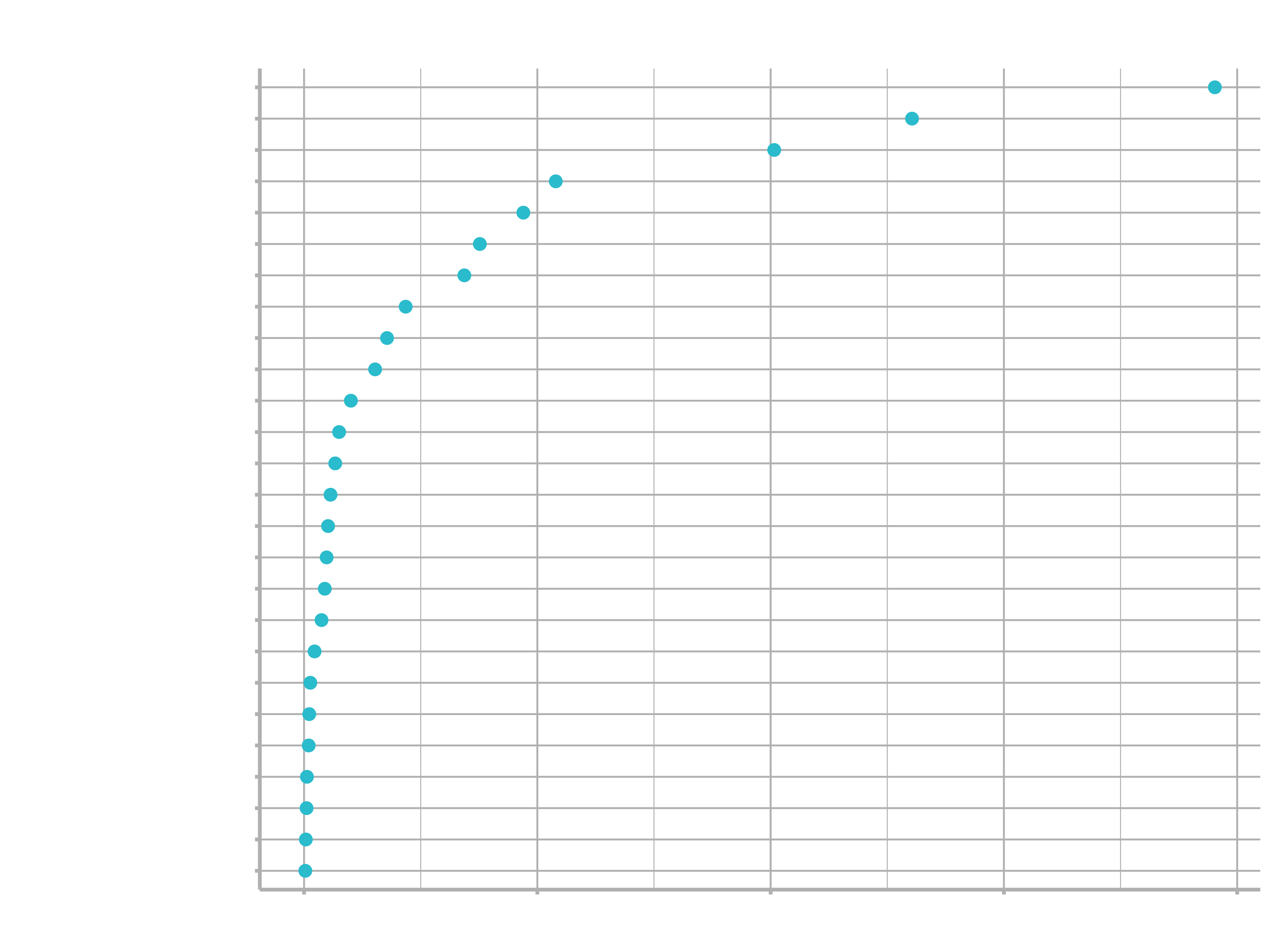
Now we do not get euro values anymore to see which features are contributing the most or the least. We do not know anymore how that model was being created. We only know that some features are more important than others, but we don’t know by how much. It is not interpretable by that standpoint.
3.2.2 randomForest - Model 06
3.2.2.1 Model
It operats simlarly to the ranger package, but it does have some differences.
# 4.2.3 Model randomForest ----
?rand_forest()
?randomForest::randomForest

set.seed(1234)
model_06_rand_forest_randomForest <- rand_forest("regression") %>%
    set_engine("randomForest") %>%

    # All character variables have to be changed to factor variables
    fit(price ~ ., data = train_tbl %>% select(-c(id:weight), -category_1, -c(category_3:gender)) %>% mutate_if(is.character, as_factor))

model_06_rand_forest_randomForest %>% calc_metrics(test_tbl)
## # A tibble: 3 x 3
##   .metric .estimator .estimate
##   <chr>   <chr>          <dbl>
## 1 rmse    standard    963.
## 2 rsq     standard       0.758
## 3 mae     standard     773.
Try to improve. There are some further features to tune. Now that we have a model, we can do the same thing that we did before with ranger. We can compute the feature importance with randomForest::importance(). It works pretty similar.
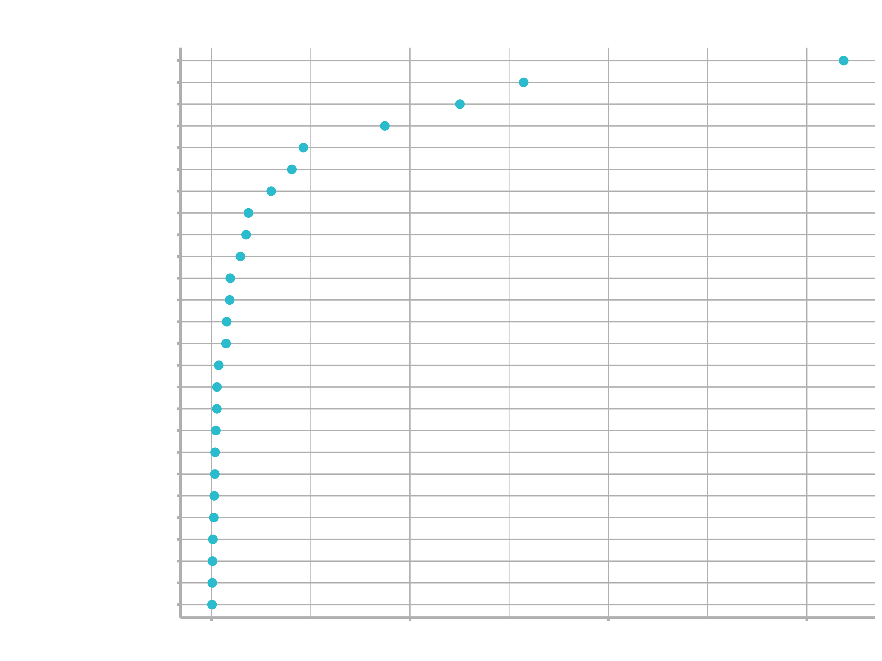
3.2.2.2 Model Explanation
as_tibble(): Convert an object to a tibble. Provide a name for the rownames argument to preserve the names. We could have used this approach with the vector as well instead of using enframe(). There are always several ways to accomplish a data manipulation in R.
# 4.2.4 randomForest: Feature Importance ----

model_06_rand_forest_randomForest$fit %>%
    randomForest::importance() %>%
    # Convert matrix to tibble
    as_tibble(rownames = "name") %>%
    arrange(desc(IncNodePurity)) %>%
    mutate(name = as_factor(name) %>% fct_rev()) %>%

    ggplot(aes(IncNodePurity, name)) +
    geom_point() +
    labs(
        title = "randomForest: Variable Importance",
        subtitle = "Model 06: randomForest Model"
    )
3.3 Gradient Boosting Machines (GBM) - Model 7
The Gradient Boosting Machine, or GBM, is another tree-based model that has many advantages including being both extremely fast and powerful. We will implement the XGBoost algorithm, which is an algorithm popularized by Kaggle for winning many challenges. Here are several videos from StatQuest that provide theory on Gradient Boosting.
Decision Trees & XGBoost in 2 Minutes
This video comes from 2-Minute Papers. It covers the general idea of building lots of “weak learners”, the aggregation strategy that XGBoost uses.
Gradient Decent
Gradient Decent is how the Gradient Boosting Machine (GBM) works. Key concept - Understanding the Learning Rate.
AdaBoost
Adaptive Boosting - aka AdaBoost - Was the first form of GBM developed. It’s a precursor to XGBoost, the popular algorithm that most data scientists now use for GBMs.
3.3.1 Model - XGBoost
Set up the parsnip model specification for boosted trees (GBMs)
?boost_tree
We have almost the same arguments like the decision trees / randomForest. The new ones are learn_rate, loss_reduction and sample_size. The learning rate is probably the most powerful. The gradient decent learning rate is used to find the global optima that reduces the model error (loss function). Too low, and algorithm gets stuck in a local optima. Too high, and it misses the global optima.
The engine we are using is xgboost:
?xgboost::xgboost
There are a lot of parameters in the params argument. There are two different type of boosters: TreeBooster and Linear Booster. We are focusing on the first one.
# 4.3 XGBOOST ----
# 4.3.1 Model ----

set.seed(1234)
model_07_boost_tree_xgboost <- boost_tree(
    mode = "regression",
    mtry = 30,
    learn_rate = 0.25,
    tree_depth = 7
    ) %>%
    set_engine("xgboost") %>%
    fit(price ~ ., data = train_tbl %>% select(-c(id:weight), -category_1, -c(category_3:gender)))

model_07_boost_tree_xgboost %>% calc_metrics(test_tbl)
## # A tibble: 3 x 3
##   .metric .estimator .estimate
##   <chr>   <chr>          <dbl>
## 1 rmse    standard    1021.
## 2 rsq     standard       0.726
## 3 mae     standard     793.
Try to improve.
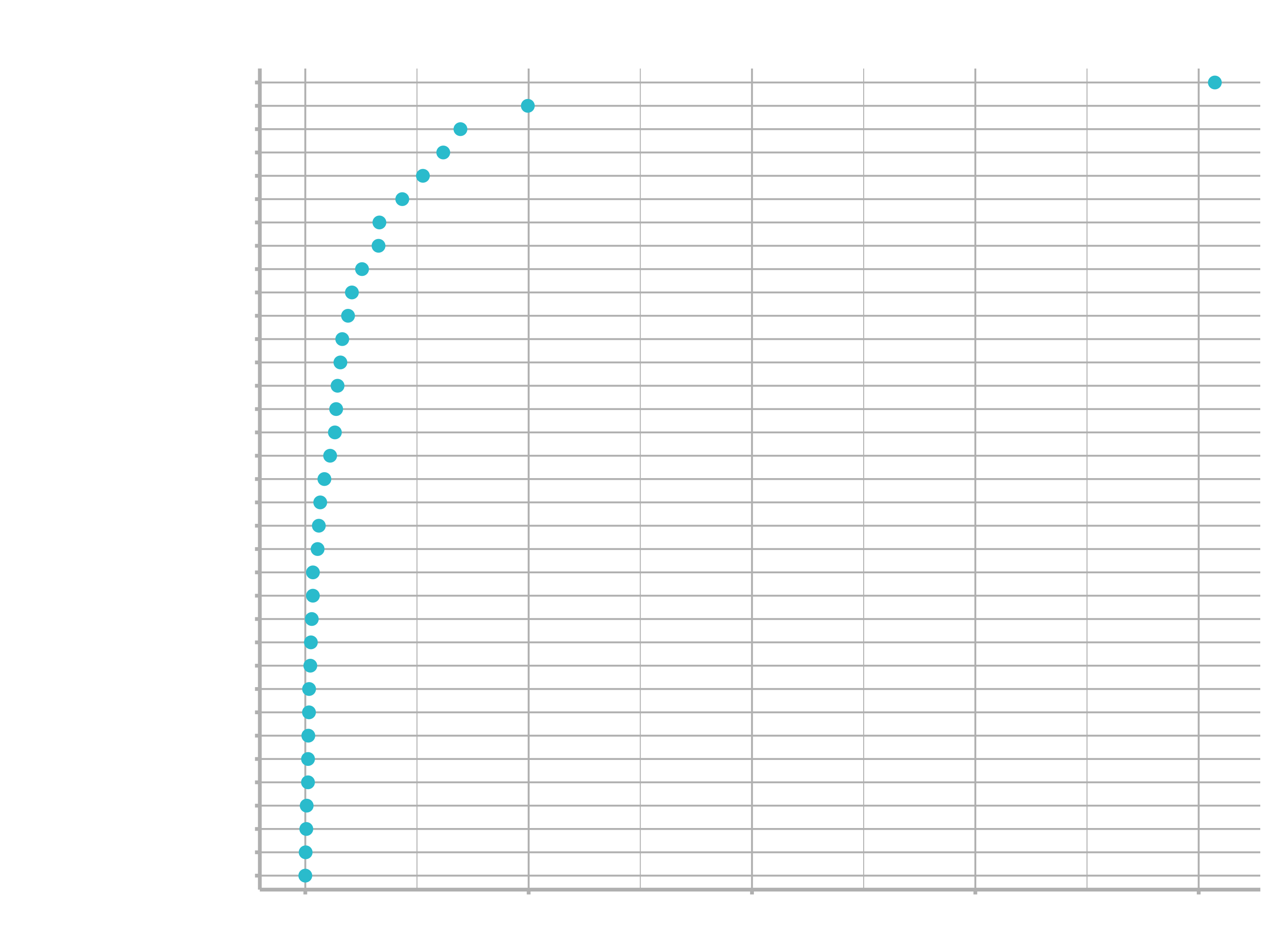
3.3.2 Model Explanation
?xgboost::xgb.importance
# 4.3.2 Feature Importance ----

model_07_boost_tree_xgboost$fit %>%
    xgboost::xgb.importance(model = .) %>%
    as_tibble() %>%
    arrange(desc(Gain)) %>%
    mutate(Feature = as_factor(Feature) %>% fct_rev()) %>%

    ggplot(aes(Gain, Feature)) +
    geom_point() +
    labs(
        title = "XGBoost: Variable Importance",
        subtitle = "Model 07: XGBoost Model"
    )
4. Prediction & Evaluation
Now we want to test those algorithms out. We want to see how these models generalize to totally unseen bike models and see if it passes the common sense test.
But on of the issues, we ran into already …
… we actually trained these models by using that hold-out (test) set to adjust the parameters. This is never a good idea, but for the purpose of an introduction it is alright, since we did not mention cross validation and so on.
It’s always a good idea to set up an experiment to determine if your models are predicting how you think they should predict. Use visualization to help determine model effectiveness and performance. Plot the other bikes prices and compare them to the prices of our models.
# 5.0 TESTING THE ALGORITHMS OUT ----
g1 <- bike_features_tbl %>%
    mutate(category_2 = as.factor(category_2) %>%
           fct_reorder(price)) %>%

    ggplot(aes(category_2, price)) +
    geom_violin() +
    geom_jitter(width = 0.1, alpha = 0.5, color = "#2dc6d6") +
    coord_flip() +
    facet_wrap(~ frame_material) +
    scale_y_continuous(labels = scales::dollar_format()) +
    labs(
        title = "Unit Price for Each Model",
        y = "", x = "Category 2"
    )
We want to bring a Cyclo-Cross bike with an aluminium frame and a Shimano XT groupset to market. Let’s create it:
# 5.1 NEW MODEL ----

new_cross_country <- tibble(
        model = "Exceed AL SL new",
        category_2 = "Cross-Country",
        frame_material = "aluminium",
        shimano_dura_ace = 0,
        shimano_ultegra = 0,
        shimano_105 = 0,
        shimano_tiagra = 0,
        Shimano_sora = 0,
        shimano_deore = 0,
        shimano_slx = 0,
        shimano_grx = 0,
        Shimano_xt = 1,
        Shimano_xtr = 0,
        Shimano_saint = 0,
        SRAM_red = 0,
        SRAM_force = 0,
        SRAM_rival = 0,
        SRAM_apex = 0,
        SRAM_xx1 = 0,
        SRAM_x01 = 0,
        SRAM_gx = 0,
        SRAM_nx = 0,
        SRAM_sx = 0,
        Campagnolo_potenza = 0,
        Campagnolo_super_record = 0,
        shimano_nexus = 0,
        shimano_alfine = 0
)

new_cross_country
Predict the price model by model…
# Linear Methods ----
# Doesn't work right now
predict(model_01_linear_lm_simple,, new_data = new_cross_country)
## # A tibble: 1 x 1
##   .pred
##   <dbl>
## 1 2323.
# Tree-Based Methods ----

predict(model_07_boost_tree_xgboost, new_data = new_cross_country)
## # A tibble: 1 x 1
##   .pred
##   <dbl>
## 1 2376.
… or all at once. Data frames can be a very useful way to keep models organized. Just put them in a “list-column”:
# Iteration
models_tbl <- tibble(
    model_id = str_c("Model 0", 1:7),
    model = list(
        model_01_linear_lm_simple,
        model_02_linear_lm_complex,
        model_03_linear_glmnet,
        model_04_tree_decision_tree,
        model_05_rand_forest_ranger,
        model_06_rand_forest_randomForest,
        model_07_boost_tree_xgboost
    )
)

models_tbl

# Add Predictions

predictions_new_cross_country_tbl <- models_tbl %>%
    mutate(predictions = map(model, predict, new_data = new_cross_country)) %>%
    unnest(predictions) %>%
    mutate(category_2 = "Cross-Country") %>%
    left_join(new_cross_country, by = "category_2")

predictions_new_cross_country_tbl
Each geom has a data argument. Overwriting the data argument is a way to add new data to the plot.
# Update plot

g2 <- g1 +
    geom_point(aes(y = .pred), color = "red", alpha = 0.5,
               data = predictions_new_cross_country_tbl) +
    ggrepel::geom_text_repel(aes(label = model_id, y = .pred),
                             size = 3,
                             data = predictions_new_cross_country_tbl)
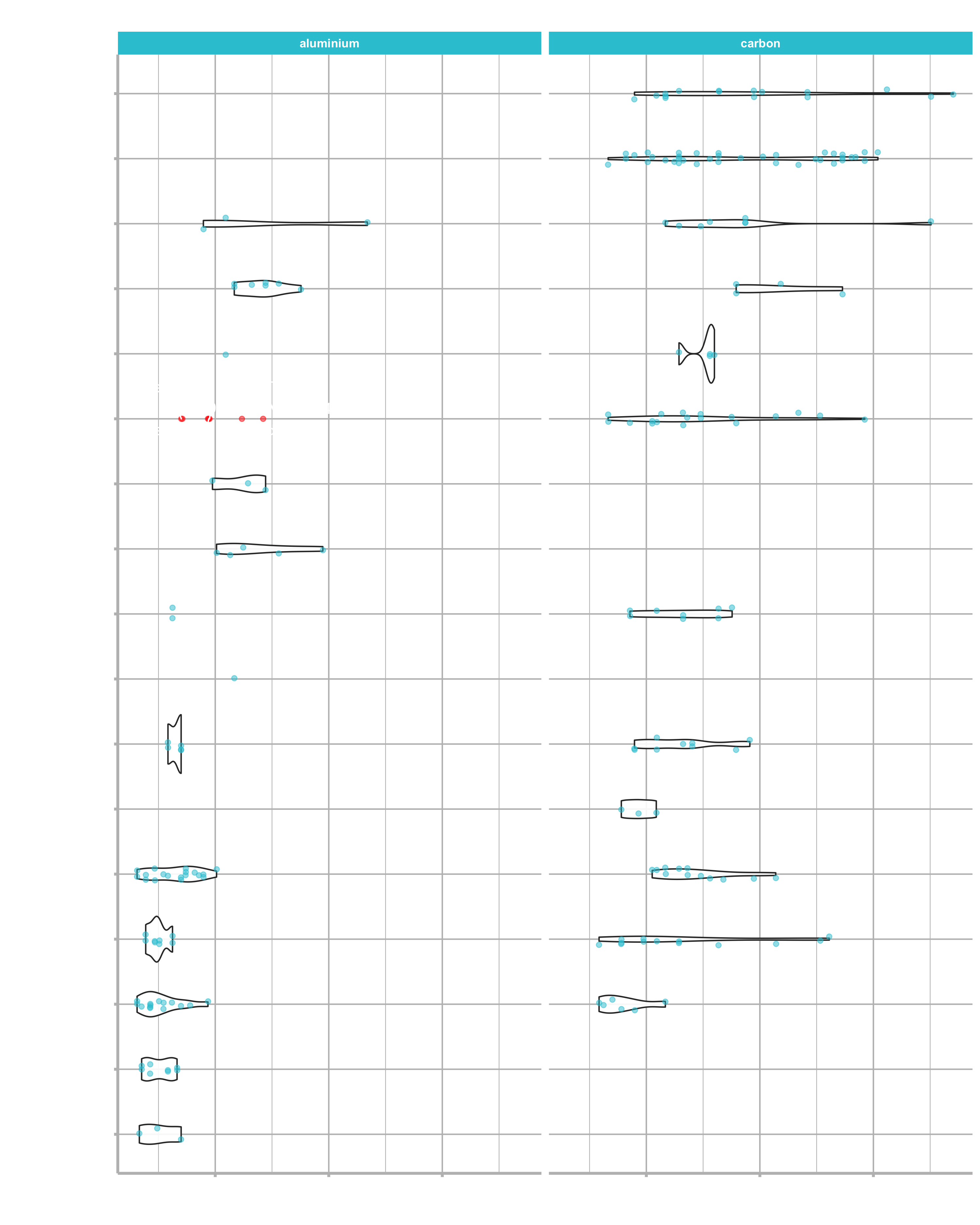
I leave the interpretation to you!
Challenge
In this session we did not use the recipes packages to prepare our data. This is going to be your challenge. For further information take a look at the last session or just use google. Prepare the data for the models with the steps provided below. Remember, you don’t need to set the flags by yourself (see all_nominal()).
I. Build a model
II. Create features with the recipes package
This is just a template. Check the documentation for further information.
?recipe
?step_dummy
?prep
?bake

recipe_obj <- recipe(...) %>%
                step_rm(...) %>%
                step_dummy(... ) %>% # Check out the argument one_hot = T
                prep()

train_transformed_tbl <- bake(..., ...)
test_transformed_tbl  <- bake(..., ...)
III. Bundle the model and recipe with the workflow package
IV. Evaluate your model with the yardstick package
Just use the function, that we have created in this session.