Data Wrangling
Data wrangling (Cleaning & Preparation) is the important process of preparing data for analysis and the foundation of exploratory data analysis. We prepare data prior to modeling & machine learning. In this session we will repeat most of the data wrangling function we have discussed already earlier. After that the concept of data.table for handling big data will be introduced.
Theory Input
Recap / Practice
The functions for data wrangling you need to learn are integrated into 7 Key Topics:
- Working with columns
(features)- Subsetting and reorganizing columns - Working with rows
(observations)- Filtering rows - Performing
feature-based calculations- using mutate() - Performing
summary calculations- Working with groups and summarized data Reshapingdata (pivoting) - Converting from wide to long format and vice versaCombiningJoining & Binding dataSplitting & CombiningBuilding features from text columns
We have used already most of the functions in the last sessions. However, in order to learn them you need to practice them. Let’s see if you can solve the following tasks. We start with the bikes_tbl from the last Canyon case. First we have to replace the dots with the underscores and split the category column (same steps we have applied to bike_orderlines_tbl).
bikes_tbl <- read_excel("00_data/01_bike_sales/01_raw_data/bikes.xlsx") %>%
                  # Separate product category name in main and sub
                  separate(col    = category,
                           into   = c("category.1", "category.2", "category.3"),
                           sep    = " - ") %>%
                  # Renaming columns
                  set_names(names(.) %>% str_replace_all("\\.", "_"))
(1) Basic column operations
Working with columns/features
Functions: select(), pull(), rename() and set_names()
1.1 Basic select(): Use select() in three different ways (column names, indices and select_helpers) to select the first 3 columns.
bikes_tbl %>%
  select(bike_id, model, model_year)
bikes_tbl %>%
  select(1:3)
bikes_tbl %>%
  select(1, contains("model"))
1.2 Reduce columns: Select only model and price:
bikes_tbl %>%
    select(model, price)
1.3 Rearrange columns: Put the category columns in front (select_helpers):
bikes_tbl %>%
  select(category_1:category_3, everything())
# Alternative using relocate()
bikes_tbl %>%
  relocate(category_1:category_3)
1.4 Select helpers: Select all columns that start with model:
?starts_with
bikes_tbl %>%
  select(starts_with("model"))
1.5 Pull() extracts content of a tibble column. Calculate the mean auf price:
bikes_tbl %>%
  # select(price) %>% Does not work
  pull(price) %>%
  mean()
1.6 Select() and where(): First extract all character columns. Then extract all non numeric columns.
?where
bikes_tbl %>%
    select(where(is.character))
bikes_tbl %>%
    select(where(is.numeric))
bikes_tbl %>%
    select(!where(is.numeric))
1.7 Select model, category_1, category_2, category_3, price and rename them to Model, Bike Family, Ride Style, Bike Category, Price in Euro. Use rename() to rename one column at a time.
bikes_tbl %>%
    select(model, category_1, category_2, category_3, price) %>%
    rename(
        Model           = model,
        `Bike Family`   = category_1,
        `Ride Style`    = category_2,
        `Bike Category` = category_3,
        `Price in Euro` = price
    )
1.8 Select model, category_1, category_2, category_3, price and rename them to Model, Bike Family, Ride Style, Bike Category, Price in Euro. Use set_names() to rename all columns at once.
bikes_tbl %>%
    select(model, category_1, category_2, category_3, price) %>%
    set_names(c("Model", "Bike Family", "Ride Style", "Bike Category", "Price in Euro"))
# An example using str_replace
bikes_tbl %>%
    select(model, category_1, category_2, category_3, price) %>%
    set_names(names(.) %>% str_replace("_", " ") %>% str_to_title())
(2) Basic row operations
Working with rows/observations
Functions: arrange(), filter(), slice() and distinct()
2.1 Arranging with arrange() and desc(): Select model and price and arrange the data by price in a descending order:
bikes_tbl %>%
    select(model, price) %>%
    arrange(desc(price)) %>%
    View()
2.2 Filtering rows. Formula based with filter():2.2.1 Filter rows, where price is greater than the mean of price:
bikes_tbl %>%
    select(model, price) %>%
    filter(price > mean(price))
2.2.2 Filter rows, where price is greater 5000 or lower 1000 and sort by descending price:
bikes_tbl %>%
  select(model, price) %>%
  filter((price > 5000) | (price < 1000)) %>%
  arrange(desc(price)) %>%
  View()
2.2.3 Filter rows, where price is greater 5000 and the model contains “Endurace” (str_detect()):
bikes_tbl %>%
    select(model, price) %>%
    filter(price > 5000,
           model %>% str_detect("Endurace")
           )
2.2.4 Filter rows, where the category_1 is “Hybrid / City” or “E-Bikes”. Use the %in% operator:
bikes_tbl %>%
    filter(category_1 %in% c("Hybrid / City", "E-Bikes"))
2.2.5 Filter rows, where the category_2 is “E-Mountain”:
bikes_tbl %>%
    filter(category_2 == "E-Mountain")
2.2.6 Negate 2.2.4 and 2.2.5
bikes_tbl %>%
    filter(category_2 != "E-Mountain")
bikes_tbl %>%
    filter(!(category_2 %in% c("Hybrid / City", "E-Bikes")))
2.3 Filtering rows with row number(s) using slice():2.3.1 Arrange by price (1. ascending and 2. descending) and filter the first 5 rows:
bikes_tbl %>%
    arrange(desc(price)) %>%
    slice(1:5)
bikes_tbl %>%
    arrange(price) %>%
    slice(1:5)
2.3.2 Arrange by price (descending) and filter the last 5 rows (use nrow()):
bikes_tbl %>%
    arrange(desc(price)) %>%
    slice((nrow(.)-4):nrow(.))
2.4 distinct(): Unique values. List unique values for category_1, for a combination of category_1 and category_2 and for combination of category_1, category_2 and category_3:
bikes_tbl %>%
    distinct(category_1)
bikes_tbl %>%
    distinct(category_1, category_2)
bikes_tbl %>%
    distinct(category_1, category_2, category_3)
(3) Column transformations
Performing column/feature-based calculations/transformations
Functions: mutate(), case_when(). Let’s load bike_orderlines_tbl.
bike_orderlines_tbl <- read_rds("00_data/01_bike_sales/02_wrangled_data/bike_orderlines.rds")
3.1 Adding Columns. Add the column “freight_costs”. The costs are 2 € per kilogram.
bike_orderlines_tbl %>%
    mutate(freight_costs = 2 * weight)
3.2 Overwrite Columns. Replace total_price with the log values of it:
bike_orderlines_tbl %>%
    mutate(total_price = log(total_price))
3.2 Transformations: Add the log and the square root of the total_price:
bike_orderlines_tbl %>%
    mutate(price_log = log(total_price)) %>%
    mutate(price_sqrt = total_price^0.5)
3.3 Adding Flags (feature engineering): Add a column that equals to TRUE if model contains the word “strive” and filter by that:
bike_orderlines_tbl %>%
    mutate(is_strive = model %>% str_to_lower() %>% str_detect("strive")) %>%
    filter(is_strive)
3.4 Binning with ntile(): Add a column and create 3 groups for total_price, where the groups each have as close to the same number of members as possible
bike_orderlines_tbl %>%
    mutate(price_binned = ntile(total_price, 3)) %>%
    select(total_price, price_binned, everything())
3.5 More flexible binning with case_when(): Numeric to categorical. Add a column, use case_when and choose the quantiles yourself (use quantile()). Set the results to High, Medium and Low:
bike_orderlines_tbl %>%
    mutate(price_binned = ntile(total_price, 3)) %>%
    mutate(price_binned2 = case_when(
        total_price > quantile(total_price, 0.75) ~ "High",
        total_price > quantile(total_price, 0.25) ~ "Medium",
        TRUE ~ "Low" # Everything else
    )) %>%
    select(total_price, price_binned, price_binned2, everything())
3.6 More flexible binning with case_when(): Text to categorical. Add a column that equals to “Aeroad”, when model contains “aerorad”, “Ultimate”, when model contains “ultimate” and “Not Aeroad or Ultimate” in every other case:
bike_orderlines_tbl %>%
    mutate(bike_type = case_when(
        model %>% str_to_lower() %>% str_detect("aeroad") ~ "Aeroad",
        model %>% str_to_lower() %>% str_detect("ultimate") ~ "Ultimate",
        TRUE ~ "Not Aeroad or Ultimate" # Everything else
    )) %>%
    select(bike_type, everything())
(4) Summary calculations
Functions: group_by() and summarise()
4.1 Summarise the total revenue:
bike_orderlines_tbl %>%
    summarise(
        revenue = sum(total_price)
    )
4.2 Summarise the total revenue for each category_1
bike_orderlines_tbl %>%
    group_by(category_1) %>%
    summarise(revenue = sum(total_price))
4.3 Summarise the total revenue for the groups made of category_1 and category_2. Sort by descending revenue:
bike_orderlines_tbl %>%
    group_by(category_1, category_2) %>%
    summarise(revenue = sum(total_price)) %>%
    # Always ungroup() after you summarise(). Left-over groups will cause difficult-to-detect errors.
    ungroup() %>%
    arrange(desc(revenue))
4.4 Summary functions: Group by category_1 and category_2 and summarize the price by
- count
- average
- median
- standard deviation
- minimum
- maximum
bike_orderlines_tbl %>%
    group_by(category_1, category_2) %>%
    summarise(
        count = n(),
        avg   = mean(total_price),
        med   = median(total_price),
        sd    = sd(total_price),
        min   = min(total_price),
        max   = max(total_price)
    ) %>%
    ungroup() %>%
    arrange(desc(count))
4.5 across() - Detect missing values:
# Create total_price column and insert missing values for demonstration
bike_orderlines_missing <- bike_orderlines_tbl %>%
    mutate(total_price = c(rep(NA, 4), total_price[5:nrow(.)]))
across() makes it easy to apply the same transformation to multiple columns. Use it in combination with summarise() to list missing values (absolute and relative). across() supersedes the family of “scoped variants” like summarise_at(), summarise_if(), and summarise_all(). The same applies to the family of mutate_() functions.
# detect missing (absolute)
bike_orderlines_missing %>%
    summarise(across(everything(), ~sum(is.na(.))))
# detect missing (relative)
bike_orderlines_missing %>%
    summarise(across(everything(), ~sum(is.na(.)) / length(.)))
# Handling missing data
bike_orderlines_missing %>%
    filter(!is.na(total_price))
(5) Reshaping/Pivoting
Functions: pivot_wider() and pivot_longer()
The wide format is reader-friendly. People tend to read data as wide format, where columns are categories and the cell contents are values.
5.1 pivot_wider(): Long to wide.
bike_data_sizes_tbl. Make the values of the column “size” to columns:
bike_data_sizes_tbl %>%
  select(name, year, price_euro, color, size, stock_availability) %>%
  pivot_wider(names_from  = size,
              values_from = stock_availability)
5.2 Create a tibble with the sales for each category_1 and each bikeshop. Name it bikeshop_revenue_tbl:
bikeshop_revenue_tbl <- bike_orderlines_tbl %>%
    select(bikeshop, category_1, total_price) %>%
    group_by(bikeshop, category_1) %>%
    summarise(sales = sum(total_price)) %>%
    ungroup() %>%
    arrange(desc(sales))
Make the values of category_1 to columns and make the values to a euro format (use scales::dollar(x, big.mark = ".", decimal.mark = ",", prefix = "", suffix = " €")). Store the result in bikeshop_revenue_formatted_tbl:
bikeshop_revenue_formatted_tbl <- bikeshop_revenue_tbl %>%
                                    pivot_wider(names_from  = category_1,
                                                values_from = sales) %>%
                                    mutate(
                                        Mountain = scales::dollar(Mountain, big.mark = ".", decimal.mark = ",", prefix = "", suffix = " €"),
                                        Gravel = scales::dollar(Gravel, big.mark = ".", decimal.mark = ",", prefix = "", suffix = " €"),
                                        Road     = scales::dollar(Road, big.mark = ".", decimal.mark = ",", prefix = "", suffix = " €"),
                                        `Hybrid / City` = scales::dollar(`Hybrid / City`, big.mark = ".", decimal.mark = ",", prefix = "", suffix = " €"),
                                        `E-Bikes` = scales::dollar(`E-Bikes`, big.mark = ".", decimal.mark = ",", prefix = "", suffix = " €")
                                    )
5.3 pivot_longer(): Wide to Long. Recreate the original tibble from bikeshop_revenue_formatted_tbl:
bikeshop_revenue_formatted_tbl %>%
    pivot_longer(cols           = c(names(.)[2:6]),
                 names_to       = "category_1",
                 values_to      = "sales",
                 values_drop_na = T) %>%
    mutate(sales =  sales %>% str_remove_all("€|\\.") %>% as.double())
(6) Joining & Binding
Combining data by rows/columns
Functions: left_join(), bind_cols() and bind_rows()
6.1 Create two tibbles
order_dates_tbl <- bike_orderlines_tbl %>% select(1:3)
order_items_tbl  <- bike_orderlines_tbl %>% select(1:2,4:8)
Bind them back together using left_join():
order_dates_tbl %>%
    # By argument not necessary, because both tibbles share the same column names
    left_join(y = order_items_tbl, by = c("order_id" = "order_id", "order_line" = "order_line"))
6.2 bind_cols(): Remove all columns from bike_orderlines_tbl that contain “category” but bind back the column category_1:
bike_orderlines_tbl %>%
    select(-contains("category")) %>%
    bind_cols(
        bike_orderlines_tbl %>% select(category_1)
    )
6.3 bind_rows(): Can be useful for splitting a dataset into a training and a test dateset.
train_tbl <- bike_orderlines_tbl %>%
    slice(1:(nrow(.)/2))
test_tbl <- bike_orderlines_tbl %>%
    slice((nrow(.)/2 + 1):nrow(.))
Bind them back together using bind_rows().
train_tbl %>%
    bind_rows(test_tbl)
(7) Splitting & Combining
Perform operations on text columns
Functions: separate() and unite()
Select order_date and convert it to character. Then separate it into year, month and day. Make each column numeric. Combine them again using unite() and convert the column back to a Date format (as.Date())
bike_orderlines_tbl %>%
  select(order_date) %>%
  mutate(order_date = as.character(order_date)) %>%
  # separate
  separate(col  = order_date,
           into = c("year", "month", "day"),
           sep  = "-", remove = FALSE) %>%
  mutate(
    year  = as.numeric(year),
    month = as.numeric(month),
    day   = as.numeric(day)
  ) %>%
  # unite
  unite(order_date_united, year, month, day, sep = "-", remove = FALSE) %>%
  mutate(order_date_united = as.Date(order_date_united))
data.table
The data.table is an enhanced alternative to R’s default data.frame or tibble from the tidyverse to handle tabular data. The reason it’s so popular is because it allows you to do blazing fast data manipulations (see benchmarks on up to two billion rows). This package is being used in different fields such as finance and genomics and is especially useful for those of you that are working with large data sets (for example, 1GB to 100GB in RAM). Though data.table provides a slightly different syntax from the regular R data.frame, it is quite intuitive.
The next sections will explain you the fundamental syntax of data.table and the structure behind it. All the core data manipulation functions of data.table, in what scenarios they are used and how to use it, with some advanced tricks and tips as well.
First steps
1. Installation
You can install and load the data.table package like every other package.
2. Importing data
The fread() function, short for fast read, is data.tables version of read_csv(). Like read_csv() it works for a file in your local computer as well as file hosted on the internet. Plus it is at least 20 times faster.
library(data.table)
url <- "https://opendata.ecdc.europa.eu/covid19/casedistribution/csv"
covid_data_dt <- fread(url)
class(covid_data_dt)
##  "data.table" "data.frame"
As you see from the output above, the data.table inherits from a data.frame class and therefore is a data.frame by itself. So, functions that accept a data.frame will work just fine on data.table as well (like data.frame and tibbles). When the number of rows to print exceeds the default of 100, it automatically prints only the top 5 and bottom 5 rows.
If you want to compare the speed to base R read.csv() or read_csv() from the readr package, you can run the following code:
# Create a large .csv file
test_df <- data.frame(matrix(runif(10000000), nrow=1000000))
write.csv(test_df, 'test_df.csv', row.names = F)
# Time taken by read.csv to import
system.time({test_df_base <- read.csv("test_df.csv")})
# Time taken by read_csv to import
system.time({test_df_readr <- read_csv("test_df.csv")})
# Time taken by fread to import
system.time({test_dt <- fread("test_df.csv")})
data.table is about 20x faster than base R. The time difference gets wider when the filesize increases.
You can create a data.table with the data.table() function just like a data.frame:
test_dt <- data.table(ID = c("b","b","b","a","a","c"),
                      a  = 1:6,
                      b  = 7:12,
                      c  = 13:18)
You can also convert existing objects to a data.table using setDT() and as.data.table(). The difference between the two approaches is: as.data.table(DF) function will create a copy of DF and convert it to a data.table. Whereas, setDT(DF) converts it to a data.table inplace. That means, the DF itself gets converted to a data.table and you don’t have to assign it to a different object. As a result, there is no copy made and no duplication of the same data.
Important: data.table does not have any rownames. So if the data.frame has any rownames, you need to store it as a separate column before converting to data.table. You can extract them with the function rownames().
In contrast to a data.frame or tibble, you can do a lot more than just subsetting rows and selecting columns within the frame of a data.table. To understand it we will have to first look at the general form of data.table syntax, as shown below:
## FROM[WHERE, SELECT/ORDER BY/UPDATE, GROUP BY]
covid_data_dt[i, j, by]
# Example (filter by year, sum cases, group by continent)
covid_data_dt[year == 2019, sum(cases), by = continentExp]
Users who have an SQL background might perhaps immediately relate to this syntax. The way to read it (out loud) is: Take the data.table covid_data_dt, subset/reorder rows using i, then calculate j, grouped by by. Let’s begin by looking at i and j first - subsetting rows and operating on columns.
Basic row/column operations
3. Subset and order rows in i
- Filtering rows based on conditions: Get all rows/observations for Germany in June:
covid_data_dt[countriesAndTerritories == "Germany" &
              lubridate::month(dateRep, label = T, abbr = F) == "June"]
Within the frame of a data.table, columns can be referred to as if they are variables, much like in SQL or Stata. Therefore, we simply refer to dateRep and countriesAndTerritories as if they are variables. We do not need to add the prefix covid_data_dt$ each time. Nevertheless, using covid_data_dt$dateRep would work just fine.
The row indices that satisfy the condition countriesAndTerritories == "Germany" and lubridate::month(dateRep, label = T, abbr = F) == "June" are computed, and since there is nothing else left to do, all columns from covid_data_dt at rows corresponding to those row indices are simply returned as a data.table. A comma after the condition in i is not required. But it would work just fine. In data.frames, however, the comma is necessary.
- Get the first two rows:
covid_data_dt[1:2]In this case, there is no condition. The row indices are already provided in i. We therefore return a data.table with all columns from covid_data_dt at rows for those row indices.
- Sort
covid_data_dtfirst by columnyear,monthanddayin ascending order, and then bycountriesAndTerritoriesin descending order:
covid_data_dt[order(year, month, day, -countriesAndTerritories)]We can use - on a character columns within the frame of a data.table to sort in decreasing order.
4. Select column(s) in j and rename columns
You can select columns by name or by index. To drop them just use - or !.
# Return as a vector
covid_data_dt[,geoId]
# Select multiple columns
covid_data_dt[,c("geoId", "countriesAndTerritories")]
# Return as a data.table
covid_data_dt[,list(geoId)]
# Short form using .
covid_data_dt[,.(geoId)]
# Select multiple columns
covid_data_dt[,.(geoId, countriesAndTerritories)]
# Rename them directly
covid_data_dt[,.(CountryCode = geoId, country = countriesAndTerritories)]
# select columns named in a variable using the ..prefix
select_cols = c("cases", "deaths")
covid_data_dt[, ..select_cols]
Since columns can be referred to as if they are variables within the frame of data.tables, we directly refer to the variable we want to subset. Since we want all the rows, we simply skip i. For those familiar with the Unix terminal, the .. prefix should be reminiscent of the “up-one-level” command, which is analogous to what’s happening here – the .. signals to data.table to look for the select_cols variable “up-one-level”, i.e., in the global environment in this case.
- How to rename columns? Use
setnames(x,old,new).
# List names
colnames(covid_data_dt)
setnames(covid_data_dt, "dateRep", "date")
setnames(covid_data_dt, "countriesAndTerritories", "country")
setnames(covid_data_dt, "continentExp", "continent")
Exercise
Convert the in-built airquality dataset to a data.table. Then select Solar.R, Wind and Temp for those rows where Ozone is not missing. You’ll need the function is.na().
# List all internal data sets
data()

# Load specified data sets
data("airquality")
Solution
# Solution 1
aq_dt <- data.table(airquality)
aq_dt[!is.na(Ozone), .(Solar.R, Wind, Temp)]

# Solution 2
setDT(airquality)
airquality[!is.na(Ozone), .(Solar.R, Wind, Temp)]
5. Compute or do j
- How many days have had more than 1000 deaths in a country:
covid_data_dt[,sum(deaths > 1000)]
# to list the observations put it in i
covid_data_dt[deaths > 1000]
data.table’s j can handle more than just selecting columns - it can handle expressions, i.e., computing on columns.
6. Create new columns
data.table lets you create column from within square brackets using the := operator. This saves key strokes and is more efficient:
covid_data_dt[, deaths_per_capita := deaths / popData2019]To create multiple new columns at once, use the special assignment symbol as a function:
covid_data_dt[,  `:=`(deaths_per_capita = deaths / popData2019,
                      cases_per_capita = cases / popData2019,
                      deaths_per_cases = deaths / cases)]
# To delete a column, assign it to NULL
covid_data_dt[, deaths_per_cases := NULL]
Of course, you can also modify existing columns:
covid_data_dt[,date := lubridate::dmy(date)]Exercise
Convert the in-built mtcars dataset to a data.table. Create a new column called mileage_type that has the value high if mpg > 20 else has value low. Use the function ifelse():
Solution
data("mtcars") # step not absolutely necessary
mtcars$carname <- rownames(mtcars)
mtcars_dt <- as.data.table(mtcars)
mtcars_dt[, mileage_type := ifelse(mpg > 20, 'high', 'low')]
7. Subset in i and do in j
- Calculate the average number of new cases and deaths in Germany for the month of April
covid_data_dt[country == "Germany" & month == 4,
              .(m_cases = mean(cases),
                m_death = mean(deaths)
                )
              ]
We first subset in i to find matching row indices where countries equals “Germany” and month equals 4. We do not subset the entire data.table corresponding to those rows yet. Now, we look at j and find that it uses only two columns. And what we have to do is to compute their mean(). Therefore we subset just those columns corresponding to the matching rows, and compute their mean().
Because the three main components of the query (i, j and by) are together inside […], data.table can see all three and optimise the query altogether before evaluation, not each separately. We are able to therefore avoid the entire subset (i.e., subsetting the columns besides cases and deaths), for both speed and memory efficiency.
- On how many days did less than 1000 people die in the USA in the month of June?
covid_data_dt[country == "United_States_of_America" &
              month == 5 & deaths < 1000,
              length(day)
             ]
The function length() requires an input argument. We just needed to compute the number of rows in the subset. We could have used any other column as input argument to length() really. This type of operation occurs quite frequently, especially while grouping (as we will see in the next section), to the point where data.table provides a special symbol .N for it.
covid_data_dt[country == "United_States_of_America" &
              month == 5 & deaths < 1000,
              .N
             ]
Once again, we subset in i to get the row indices where countries equals “United_States_of_America”, month equals 5 and deaths < 1000. We see that j uses only .N and no other columns. Therefore the entire subset is not materialised. We simply return the number of rows in the subset (which is just the length of row indices). Note that we did not wrap .N with list() or .(). Therefore a vector is returned.
8. Aggregations / Grouping
We’ve already seen i and j from data.table’s general form in the previous section. In this section, we’ll see how they can be combined together with by to perform operations by group.
- How can we get the number of days where the death toll was greater than 1000 for each country?
covid_data_dt[deaths > 1000, .N, by = country]We know .N is a special variable that holds the number of rows in the current group. Grouping by countries obtains the number of rows, .N, for each group.
If we need the row numbers instead of the number of rows, use .I instead of .N. If you only need the row numbers, that meet a certain criteria, wrap the condition in brackets after the .I ( run ?special-symbols for further documentation):
covid_data_dt[,.I[deaths > 1000]]- How can we get the average death and case number for each country for each month in Europe?
covid_data_dt[continent == "Europe",
              .(mean(cases), mean(deaths)),
              by = .(country, month, year)
             ]
Since we did not provide column names for the expressions in j, they were automatically generated as V1 and V2. data.table retaining the original order of groups is intentional and by design.
Exercise
Use mtcars_dt from above. Compute the number of cars and the mean mileage for each gear type.
Solution
library(magrittr) # to use the pipe
mtcars_dt[, .(.N, mileage = mean(mpg) %>% round(2)), by=gear]
Advanced operations
9. Chaining
Let’s reconsider the task of getting the means of cases and deaths for each country:
covid_cases_means <- covid_data_dt[,.(m_cases  = mean(cases) %>% round(1),
                                      m_deaths = mean(deaths) %>% round(1)),
                                      by = .(country)
]- How can we order covid_cases_means using the columns m_death?
We can store the intermediate result in a variable, and then use order(-m_deaths) on that variable. It seems fairly straightforward. But this requires having to assign the intermediate result and then overwriting that result. We can do one better and avoid this intermediate assignment to a temporary variable altogether by chaining expressions.
covid_data_dt[, .(
                  m_cases  = round(mean(cases),  digits = 1),
                  m_deaths = round(mean(deaths), digits = 1)
                 ),
                 by = .(country)][order(-m_cases)]
We can add expressions one after another, forming a chain of operations.
- Can
byaccept expressions as well or does it just take columns?
Yes it does. As an example, if we would like to find out how many days had more than 1000 deaths but less than 1000 new cases (for every country):
covid_data_dt[, .N,
                .(
                  death_gt_1k = deaths > 1000,
                  cases_lt_1k = cases < 1000
                 )
             ]
The last row corresponds to deaths > 1000 = TRUE and cases < 1000 = TRUE. We can see, that occured 4 times (once in Bolivia, China, Ecuador and Spain). Naming of the columns is optional. You can provide other columns along with expressions, for example … by = .(death_gt_1k = deaths > 1000, cases_lt_1k = cases < 1000, year).
10. .SD
- Do we have to compute
mean()for each column individually?
It is of course not practical to have to type mean(myCol) for every column one by one. What if you had 100 columns to average mean()? Suppose we can refer to the data subset for each group as a variable while grouping, then we can loop through all the columns of that variable using the R base function lapply(). You are familiar with map() from the purrr function. In this context they can be used interchangeably.
data.table provides a special symbol, called .SD. It stands for Subset of Data. It by itself is a data.table that holds the data for the current group defined using by.
covid_data_dt[, print(.SD), by = year].SD contains all the columns except the grouping columns by default. To compute on (multiple) columns, we can then simply use lapply() or map().
covid_data_dt[, lapply(.SD, mean), by = year]You will get an error, because we do not have only numeric columns.
- How can we specify just the columns we would like to compute the
mean()on?
Using the argument .SDcols. It accepts either column names or column indices. You can also provide the columns to remove instead of columns to keep using - or ! sign as well as select consecutive columns as colA:colB and deselect consecutive columns as !(colA:colB) or -(colA:colB).
Now let us try to use .SD along with .SDcols to get the mean() of cases and deaths columns grouped by year and month.
covid_data_dt[, lapply(.SD, mean),
                by = .(year, month),
                .SDcols = c("cases", "deaths")
             ]
Using sum() instead of mean() might be rather informative in this context.
11. Keys
Let’s understand why keys can be useful and how to set it. Setting one or more keys on a data.table enables it to perform binary search, which is many order of magnitudes faster than linear search, especially for large data. As a result, the filtering operations are super fast after setting the keys. There is a side effect though. By setting a key, the data.table gets sorted by that key.
To set a key, use the setkey() function:
setkey(covid_data_dt, date, country)You can set one or multiple keys if you wish. It’s so fast making it look like nothing happened. But it internally sorted data.table with date and countries as the keys. You should see it if you print the table again.
Using keyby instead of just by you can do grouping and set the by column as a key in one go. For example, in this example we saw earlier, you can skip the chaining by using keyby instead of just by. Test that for yourself.
Once the key is set, merging data.tables is very direct.
# Create a new data.table
covid_data_EUR_dt <- covid_data_dt[ continent == "Europe",
                                    lapply(.SD, function(x) {
                                                              x %>%
                                                              mean() %>%
                                                              round(1)
                                                             }
                                           ),
                                    by = .(country),
                                    .SDcols = c("cases", "deaths")
                                   ]
# Set key
setkey(covid_data_EUR_dt, country)
key(covid_data_EUR_dt)
# Create two data.tables from that
cd_dt1 <- covid_data_EUR_dt[, .(country, cases)]
cd_dt2 <- covid_data_EUR_dt[1:20, .(country, deaths)]
# Join them
cd_dt1[cd_dt2]
This returns cd_dt1‘s rows using cd_dt2 based on the key of these data.tables. You can join them also without setting keys, if you specify the on= argument (but joining by key has some speed advantages):
# Remove keys
setkey(cd_dt1, NULL)
setkey(cd_dt2, NULL)
# Join
cd_dt1[cd_dt2, on = "country"]
# If they had different colnames
cd_dt1[cd_dt2, on = c(colA = "colB")]
# Alternatively you can use the function merge()
# Inner Join
merge(cd_dt1, cd_dt2, by='country')
# Left Join
merge(cd_dt1, cd_dt2, by='country', all.x = T)
# Outer Join
merge(cd_dt1, cd_dt2, by='country', all = T)
# If they had different colnames use by.x="colA", by.y="colB"
For more information on the different joins, click here.
If you want to add the values of cd_dt2 to cd_dt1, then it’s best to join cd_dt1 with cd_dt2 and update cd_dt1 by reference (meaning with no copy necessary at all) as follows:
cd_dt1[cd_dt2, on = "country", deaths := i.deaths]This is a better approach (in terms of memory efficiency) than using cd_dt2[cd_dt1, on = "country"] because the latter just prints the result to the console. When you want to get the results back into cd_dt1, you need to use cd_dt1 <- cd_dt2[cd_dt1, on='a'] which will give you the same result.
To merge multiple data.tables, you could use the following approach:
dt_list    <- list(cd_dt1, cd_dt2, cd_dt3)
merge_func <- function(...) merge(..., all = TRUE, by='country')
dt_merged  <- Reduce(merge_func, dt_list)
12. set() function
The set() command is an incredibly fast way to assign values to a new column.
The syntax is: set(dt, i, j, value), where i is the row number and j is the column number. As a best practice, always explicitly use integers for i and j, that is, use 10L instead of 10.
It is usually used in for-loops and is literally thousands of times faster. Yes, it is so fast even when used within a for-loop, which is proof that for-loop is not really a bottleneck for speed. It is the underlying data structure related overhead that causes for-loop to be slow, which is exactly what set() avoids. It also works on a data.frame object as well.
Below is an example to illustrate the power of set() taken from official documentation itself. The speed benchmark may be outdated, but, run and check the speed by yourself to believe it.
m  = matrix(1,nrow=100000,ncol=100)
DF = as.data.frame(m)
DT = as.data.table(m)
system.time(for (i in 1:10000) DF[i,1] <- i)
## 591 seconds
system.time(for (i in 1:10000) DT[i,V1:=i])
## 2.4 seconds  ( 246 times faster, 2.4 is overhead in [.data.table )
system.time(for (i in 1:10000) set(DT,i,1L,i))
## 0.03 seconds  ( 19700 times faster, overhead of [.data.table is avoided )
Summary
The general form of data.table syntax is:
DT[i, j, by]
We have seen so far that,
Using i:
- We can subset rows similar to a data.frame - except you don’t have to use DT$ repetitively since columns within the frame of a data.table are seen as if they are variables.
- We can also sort a data.table using order(), which internally uses data.table’s fast order for performance.
We can do much more in i by keying a data.table, which allows blazing fast subsets and joins.
Using j:
- Select columns the data.table way: DT[, .(colA, colB)].
- Select columns the data.frame way: DT[, c(“colA”, “colB”)].
- Compute on columns: DT[, .(sum(colA), mean(colB))].
- Provide names if necessary: DT[, .(sA =sum(colA), mB = mean(colB))].
- Combine with
i: DT[colA > value, sum(colB)].
Using by:
- Using by, we can group by columns by specifying a list of columns or a character vector of column names or even expressions. The flexibility of
j, combined withbyandimakes for a very powerful syntax. - by can handle multiple columns and also expressions.
- We can
keybygrouping columns to automatically sort the grouped result. - We can use
.SDand.SDcolsinjto operate on multiple columns using already familiar base functions. Here are some examples: - DT[, lapply(.SD, fun), by = …, .SDcols = …] - applies fun to all columns specified in .SDcols while grouping by the columns specified in by.
- DT[, head(.SD, 2), by = …] - return the first two rows for each group.
- DT[col > val, head(.SD, 1), by = …] - combine i along with j and by.
Business case
This case is about wrangling large data with data.table. The topic are Bank Loan Defaults.
Goal
Loan defaults cost organizations multi-millions. Therefore, we need to understand which people or institutions will default on loans, in order to prevent defaults. The data we are going to analyze is coming from Fannie Mae. Fannie Mae provides both an acquisitions file and a performance file for loans:
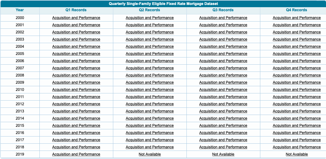
Each quarter contains around ~5M rows of data. Since 2000 that totals to around 27 GB Data. We are using the the data for the Q1 Records of 2019 (~3.1M rows). Other Quarters are even bigger. You can also download multiple quarterly data sets and merge them together if you want. But you have to register on that site. The Q1 2019 data is provided here:
We want to get that data ready for predicting defaults. Since we did not cover machine learning techniques yet, we just prepare the data and answer questions like how many loans are in each month etc.
How do we analyze this amount of data? The solutions are:
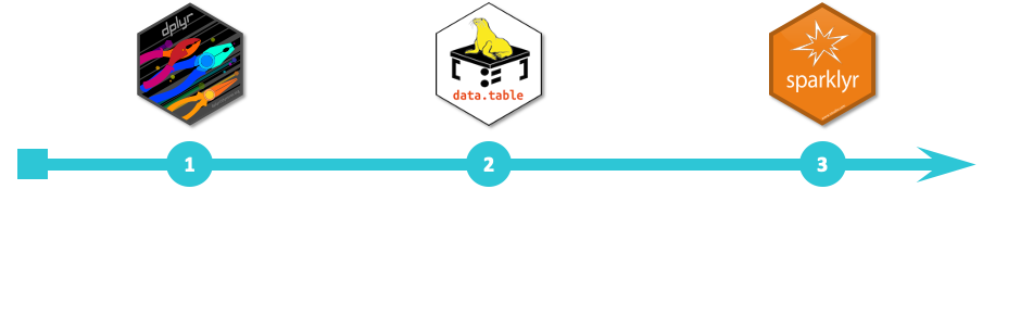
dplyr is designed for readability. It makes copies through the piping process, which is normally OK. But for large data it is not memory or speed efficient. Thus, we will be focusing on data.table, the high-performance version of base R’s data.frame, in this case. For each step, I provide a data.table and a dplyr solution, so that you can compare both approaches.
First Steps
1. Libraries
# Tidyverse
library(tidyverse)
library(vroom)
# Data Table
library(data.table)
# Counter
library(tictoc)
2. Import data
In this case we are using the package vroom, because it is even faster than data.table’s fread for reading in delimited files.
Let’s start with the acquisition data. First we need to specify the datatype of each column, that we want to import. This is necessary for datasets, that come in a weird format. So the following code is kind of a recipe for importing the data:
# 2.0 DATA IMPORT ----
# 2.1 Loan Acquisitions Data ----
col_types_acq <- list(
    loan_id                            = col_factor(),
    original_channel                   = col_factor(NULL),
    seller_name                        = col_factor(NULL),
    original_interest_rate             = col_double(),
    original_upb                       = col_integer(),
    original_loan_term                 = col_integer(),
    original_date                      = col_date("%m/%Y"),
    first_pay_date                     = col_date("%m/%Y"),
    original_ltv                       = col_double(),
    original_cltv                      = col_double(),
    number_of_borrowers                = col_double(),
    original_dti                       = col_double(),
    original_borrower_credit_score     = col_double(),
    first_time_home_buyer              = col_factor(NULL),
    loan_purpose                       = col_factor(NULL),
    property_type                      = col_factor(NULL),
    number_of_units                    = col_integer(),
    occupancy_status                   = col_factor(NULL),
    property_state                     = col_factor(NULL),
    zip                                = col_integer(),
    primary_mortgage_insurance_percent = col_double(),
    product_type                       = col_factor(NULL),
    original_coborrower_credit_score   = col_double(),
    mortgage_insurance_type            = col_double(),
    relocation_mortgage_indicator      = col_factor(NULL))
After spcifying the columns, we can import the data using the vroom function. The data is separated by |. The argument na sets the defined Values (e.g. empty values) to NA in R. That makes handling them easier.
acquisition_data <- vroom(
      file       = "loan_data/Acquisition_2019Q1.txt",
      delim      = "|",
      col_names  = names(col_types_acq),
      col_types  = col_types_acq,
      na         = c("", "NA", "NULL"))
acquisition_data %>% glimpse()
The result is a tibble with 297,452 rows. It contains the data about all the loans. Each loan is identified by an id loan_id. The data tells you, who sold the loan (e.g. JPMORGAN CHASE BANK), what is the original interest rate (e.g. 5.875 %), the original unpaid balance (e.g. 324.000 $), the loan term (e.g. 360 month / 30 years) and so on. But it does not show how the loans change over time. And that’s what the next dataset is for. The performance data. We are going to do the same process:
# 2.2 Performance Data ----
col_types_perf = list(
    loan_id                                = col_factor(),
    monthly_reporting_period               = col_date("%m/%d/%Y"),
    servicer_name                          = col_factor(NULL),
    current_interest_rate                  = col_double(),
    current_upb                            = col_double(),
    loan_age                               = col_double(),
    remaining_months_to_legal_maturity     = col_double(),
    adj_remaining_months_to_maturity       = col_double(),
    maturity_date                          = col_date("%m/%Y"),
    msa                                    = col_double(),
    current_loan_delinquency_status        = col_double(),
    modification_flag                      = col_factor(NULL),
    zero_balance_code                      = col_factor(NULL),
    zero_balance_effective_date            = col_date("%m/%Y"),
    last_paid_installment_date             = col_date("%m/%d/%Y"),
    foreclosed_after                       = col_date("%m/%d/%Y"),
    disposition_date                       = col_date("%m/%d/%Y"),
    foreclosure_costs                      = col_double(),
    prop_preservation_and_repair_costs     = col_double(),
    asset_recovery_costs                   = col_double(),
    misc_holding_expenses                  = col_double(),
    holding_taxes                          = col_double(),
    net_sale_proceeds                      = col_double(),
    credit_enhancement_proceeds            = col_double(),
    repurchase_make_whole_proceeds         = col_double(),
    other_foreclosure_proceeds             = col_double(),
    non_interest_bearing_upb               = col_double(),
    principal_forgiveness_upb              = col_double(),
    repurchase_make_whole_proceeds_flag    = col_factor(NULL),
    foreclosure_principal_write_off_amount = col_double(),
    servicing_activity_indicator           = col_factor(NULL))
performance_data <- vroom(
    file       = "loan_data/Performance_2019Q1.txt",
    delim      = "|",
    col_names  = names(col_types_perf),
    col_types  = col_types_perf,
    na         = c("", "NA", "NULL"))
performance_data %>% glimpse()
Thise data is bigger. It has 3.1M rows. It is perfect for data.table. The reason why it so big is because for each of those loans, there is a time series to it. So it characterizes the performance of that loan over time. That means: Is it getting paid? What are the numbers of month to maturity…
data.table & Wrangling
3. Convert to data.table
# 3.1 Acquisition Data ----
class(acquisition_data)
setDT(acquisition_data)
class(acquisition_data)
acquisition_data %>% glimpse()
# 3.2 Performance Data ----
setDT(performance_data)
performance_data %>% glimpse()
4. Data wrangling
4.1 Merge the data
Merge the data via the loan_id
# 4.0 DATA WRANGLING ----
# 4.1 Joining / Merging Data ----
tic()
combined_data <- merge(x = acquisition_data, y = performance_data,
                       by    = "loan_id",
                       all.x = TRUE,
                       all.y = FALSE)
toc()
combined_data %>% glimpse()
# Same operation with dplyr
tic()
performance_data %>%
  left_join(acquisition_data, by = "loan_id")
toc()
4.2 Prepare the data
Let’s set the key to loan_id to set the default grouping operator and improve the computational speed.
Let’s also ensure that the data is ordered by the loan_id first and then the monthly_reporting_period. That is important, because we are doing time series operations, where the order is crucial.
# Preparing the Data Table
setkey(combined_data, "loan_id")
key(combined_data)
?setorder()
setorderv(combined_data, c("loan_id", "monthly_reporting_period"))
4.3 Select columns
Select only the following columns:
# 4.3 Select Columns ----
combined_data %>% dim()
keep_cols <- c("loan_id",
               "monthly_reporting_period",
               "seller_name",
               "current_interest_rate",
               "current_upb",
               "loan_age",
               "remaining_months_to_legal_maturity",
               "adj_remaining_months_to_maturity",
               "current_loan_delinquency_status",
               "modification_flag",
               "zero_balance_code",
               "foreclosure_costs",
               "prop_preservation_and_repair_costs",
               "asset_recovery_costs",
               "misc_holding_expenses",
               "holding_taxes",
               "net_sale_proceeds",
               "credit_enhancement_proceeds",
               "repurchase_make_whole_proceeds",
               "other_foreclosure_proceeds",
               "non_interest_bearing_upb",
               "principal_forgiveness_upb",
               "repurchase_make_whole_proceeds_flag",
               "foreclosure_principal_write_off_amount",
               "servicing_activity_indicator",
               "original_channel",
               "original_interest_rate",
               "original_upb",
               "original_loan_term",
               "original_ltv",
               "original_cltv",
               "number_of_borrowers",
               "original_dti",
               "original_borrower_credit_score",
               "first_time_home_buyer",
               "loan_purpose",
               "property_type",
               "number_of_units",
               "property_state",
               "occupancy_status",
               "primary_mortgage_insurance_percent",
               "product_type",
               "original_coborrower_credit_score",
               "mortgage_insurance_type",
               "relocation_mortgage_indicator")
And overwrite your data.table with those selected columns:
combined_data <- combined_data[, ..keep_cols]
combined_data %>% dim()
combined_data %>% glimpse()
4.4 Grouped Mutations
Let’s work with the column current_loan_delinquency_status:
combined_data$current_loan_delinquency_status %>% unique()
##  0 NA  1  2  3  4  5  6  7  8  9 10 11 12

# or:
combined_data[,current_loan_delinquency_status] %>% unique()
##  0 NA  1  2  3  4  5  6  7  8  9 10 11 12
Zero is good. Zero means the loan is paid on time. One would mean that the borrower is one month behind and so on… The worst case is 12. For machine learning approaches we could want to add a response variable, that tells us whether a loan will become delinquent in next 3 months. For that we are using the lead() function, that finds previous values in a vector (the opposite lag() finds next values). Those functions are useful for comparing values ahead of or behind the current values.
We need a column that equals to TRUE or FALSE. Take the delinquency status, shift that value 3 units/month ahead and figure out whether or not it was greater than one. We have to do that for each loan_id. Use modify in place := to speed up the calculations.
# 4.4 Grouped Mutations ----
# - Add response variable (Predict wether loan will become delinquent in next 3 months)
# dplyr
tic()
temp <- combined_data %>%
  group_by(loan_id) %>%
  mutate(gt_1mo_behind_in_3mo_dplyr = lead(current_loan_delinquency_status, n = 3) >= 1) %>%
  ungroup()
toc()
combined_data %>% dim()
temp %>% dim()
# data.table
tic()
combined_data[, gt_1mo_behind_in_3mo := lead(current_loan_delinquency_status, n = 3) >= 1,
              by = loan_id]
toc()
combined_data %>% dim()
# Remove the temp variable
rm(temp)
Analysis & Findings
5. Analysis
Answer the following questions:
- How many loans are in each month. We have to take a look at the column
monthly_reporting_period. Watch out for NA values.
# 5.1 How many loans in a month ----
tic()
combined_data[!is.na(monthly_reporting_period), .N, by = monthly_reporting_period]
toc()
tic()
combined_data %>%
    filter(!is.na(monthly_reporting_period)) %>%
    count(monthly_reporting_period)
toc()- Which loans have the most outstanding delinquencies?
# 5.2 Which loans have the most outstanding delinquencies ----
# data.table
tic()
combined_data[current_loan_delinquency_status >= 1,
              list(loan_id, monthly_reporting_period, current_loan_delinquency_status, seller_name, current_upb)][
                , max(current_loan_delinquency_status), by = loan_id][
                  order(V1, decreasing = TRUE)]
toc()
# dplyr
tic()
combined_data %>%
  group_by(loan_id) %>%
  summarise(total_delinq = max(current_loan_delinquency_status)) %>%
  ungroup() %>%
  arrange(desc(total_delinq))
toc()- What is the last unpaid balance value for delinquent loans
# 5.3 Get last unpaid balance value for delinquent loans ----
# data.table
tic()
combined_data[current_loan_delinquency_status >= 1, .SD[.N], by = loan_id][
  !is.na(current_upb)][
  order(-current_upb), .(loan_id, monthly_reporting_period, current_loan_delinquency_status, seller_name, current_upb)
  ]
toc()
# dplyr
tic()
combined_data %>%
  filter(current_loan_delinquency_status >= 1) %>%
  filter(!is.na(current_upb)) %>%
  group_by(loan_id) %>%
  slice(n()) %>%
  ungroup() %>%
  arrange(desc(current_upb)) %>%
  select(loan_id, monthly_reporting_period, current_loan_delinquency_status, seller_name, current_upb)
toc()- What are the Loan Companies with highest unpaid balance?
# 5.4 Loan Companies with highest unpaid balance
# data.table
tic()
upb_by_company_dt <- combined_data[!is.na(current_upb), .SD[.N], by = loan_id][
  , .(sum_current_upb = sum(current_upb, na.rm = TRUE), cnt_current_upb = .N), by = seller_name][
    order(sum_current_upb, decreasing = TRUE)]
toc()
upb_by_company_dt
# dplyr
tic()
upb_by_company_tbl <- combined_data %>%
  filter(!is.na(current_upb)) %>%
  group_by(loan_id) %>%
  slice(n()) %>%
  ungroup() %>%
  group_by(seller_name) %>%
  summarise(
    sum_current_upb = sum(current_upb, na.rm = TRUE),
    cnt_current_upb = n()
  ) %>%
  ungroup() %>%
  arrange(desc(sum_current_upb))
toc()
6. Findings
- Both data.table & dplyr great for data manipulation.
- data.table is faster on grouped mutations. Speedup of 2X-10X on inplace calculations using
:=. - data.table can be slower than dplyr on grouped summarizations.
The trick to solving big data Problems. Make them small. Large datasets can be sampled. Sampling makes data manageable. Upgrade to Big Data tools once you have a good methodology.
Challenge
Patents play a critical role in incentivizing innovation, without which we wouldn’t have much of the technology we rely on everyday. What does your iPhone, Google’s PageRank algorithm, and a butter substitute called Smart Balance all have in common?
…They all probably wouldn’t be here if not for patents. A patent provides its owner with the ability to make money off of something that they invented, without having to worry about someone else copying their technology. Think Apple would spend millions of dollars developing the iPhone if Samsung could just come along and rip it off? Probably not.
Patents offer a great opportunity for data analysis, because the data is public. PatentsView is one of USPTO’s (United States Patent and Trademark Office) new initiatives intended to increase the usability and value of patent data. That data can be downloaded here:
Information about the data will be found here:
You can import the data like this:
library(vroom)
col_types <- list(
  id = col_character(),
  type = col_character(),
  number = col_character(),
  country = col_character(),
  date = col_date("%Y-%m-%d"),
  abstract = col_character(),
  title = col_character(),
  kind = col_character(),
  num_claims = col_double(),
  filename = col_character(),
  withdrawn = col_double()
)
patent_tbl <- vroom(
            file       = "patent.tsv",
            delim      = "\t",
            col_types  = col_types,
            na         = c("", "NA", "NULL")
        )
In the Patents_DB_dictionary_bulk_downloads.xlsx file you will find information about the datatypes for each column of the tables. This will help you to create the “recipe” to import the data.
To speed up your processing, you can select col_skip() as a “datatype” to only read the columns of the data into R, that you will need for your analysis.
Answer the following questions with that data:
- Patent Dominance: What US company / corporation has the most patents? List the 10 US companies with the most assigned/granted patents.
- Recent patent acitivity: What US company had the most patents granted in 2019? List the top 10 companies with the most new granted patents for 2019.
- Innovation in Tech: What is the most innovative tech sector? For the top 10 companies (worldwide) with the most patents, what are the top 5 USPTO tech main classes?
Answer the question with data.table or dplyr. You will need the following tables for each question:
| Question | Table |
|---|---|
| 1 | assignee, patent_assignee |
| 2 | assignee, patent_assignee, patent |
| 3 | assignee, patent_assignee, uspc |