Data Acquisition
Before you can start to work with your data within your R session, you need to get the data into your R workspace. Data acquisition is the process you use to import data into your R session so that it can be viewed, stored, and analyzed. We have discussed already how to import spreadsheet-like tables saved as csv or Excel files using read_csv and read_excel. Data and information on the web is growing exponentially. In today’s world, all the data that you need for your own personal projects is already available on the internet – the only thing limiting you from using it is the ability to access it. This session will cover how to connect to databases and how to acquire data from the web.
Why web scrape in the context of Business Analytics?
- The web is full of free & valuable data
- Many companies put their information out there
- Few companies have programs to actively retrieve & analyze competitor data
- Companies that implement programs have a Competitive Advantage
Theory Input
Databases
Connecting to databases is kind of an advanced topic, but it is something which is really important for you to do, because as a business analyst you are going to need to get data out of an Enterprise Resource Planning (ERP) system or customer relationship management (CRM) database quite frequently. Everything you will need is well documented here:
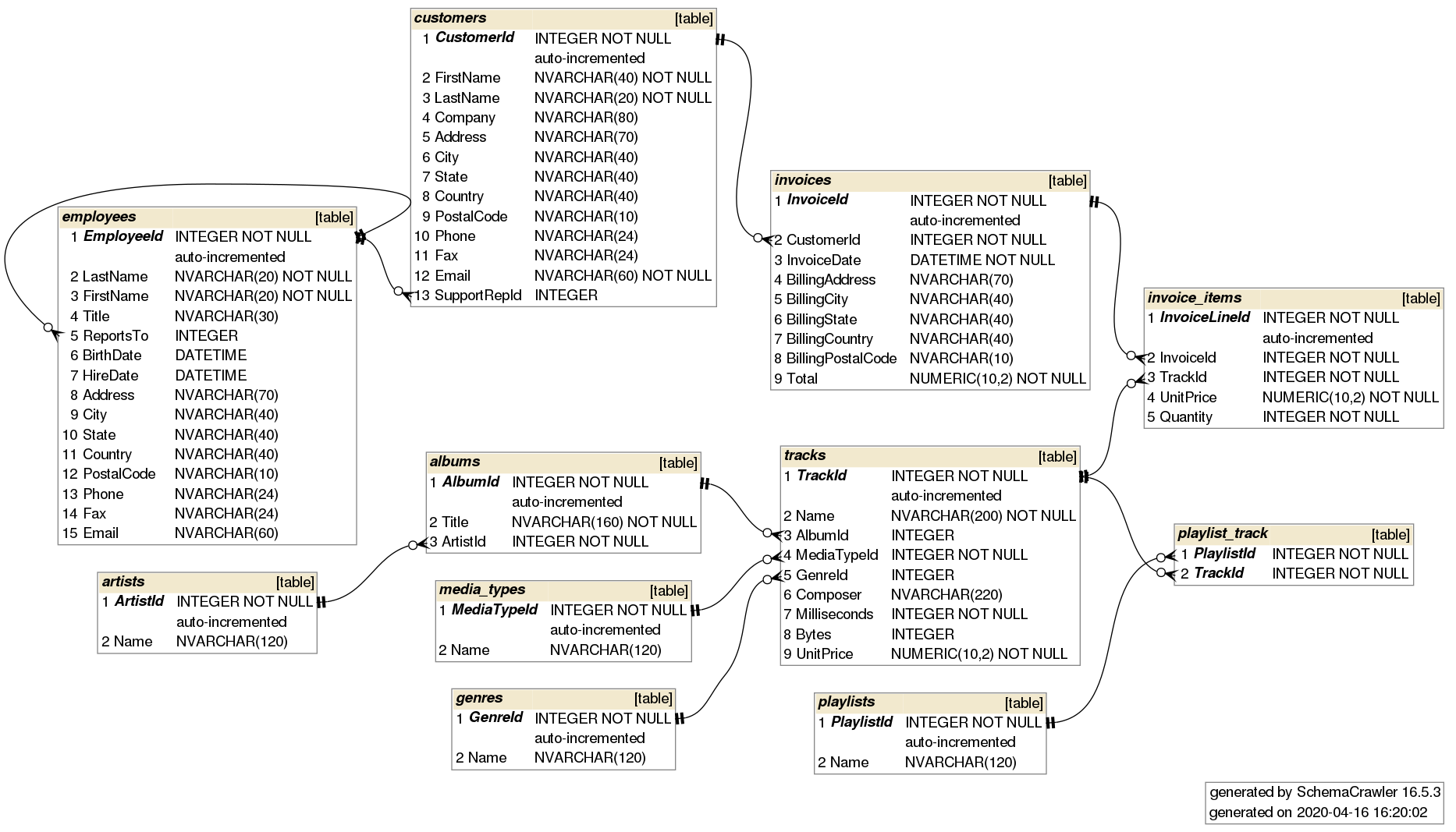
There are many different kinds of databases out there: MySQL, PostgreSQL, Redshift, etc. In the documentation you will find instructions for each of those. I will only demonstrate an example for SQLite with the Chinook database. The Chinook data model represents a digital media store, including tables for artists, albums, media tracks, invoices and customers. The database should be already present in your project folder.
To open up a connection you need the RSQLite package and the function dbConnect(). This function is used to create a connection object, which is a set of instructions for connecting to a database. It takes a couple of different arguments. The first is drv for the driver. In this case we pass the SQLite() function, which is a database driver that comes with the package. The second dbname is just the path, which points to the database.
library(RSQLite)
con <- RSQLite::dbConnect(drv    = SQLite(),
                          dbname = "00_data/02_chinook/Chinook_Sqlite.sqlite")
Once we have that connection, we can use the function dbListTables() (from the DBI package) to return the names of the tables that are available in the database that you are connected to:
dbListTables(con)
##  [1] "Album"         "Artist"        "Customer"      "Employee"
##  [5] "Genre"         "Invoice"       "InvoiceLine"   "MediaType"
##  [9] "Playlist"      "PlaylistTrack" "Track"
To examine a table from a database, use tbl() from the dplyr package. Just pass the connection object and the name of the table.
tbl(con, "Album")
## # Source:   table [?? x 3]
## # Database: sqlite 3.30.1 [~/Chinook_Sqlite.sqlite]
##    AlbumId Title                                 ArtistId
##      <int> <chr>                                    <int>
##  1       1 For Those About To Rock We Salute You        1
##  2       2 Balls to the Wall                            2
##  3       3 Restless and Wild                            2
##  4       4 Let There Be Rock                            1
##  5       5 Big Ones                                     3
##  6       6 Jagged Little Pill                           4
##  7       7 Facelift                                     5
##  8       8 Warner 25 Anos                               6
##  9       9 Plays Metallica By Four Cellos               7
## 10      10 Audioslave                                   8
## # … with more rows
This is just a connection so far. If we want to pull the data into local memory we have to chain another function called collect():
album_tbl <- tbl(con, "Album") %>% collect()If you are familiar with SQL, you can send queries like this: x <- dbGetQuery(con, 'SELECT * FROM Artist').
Once you are done with the data acquisition, disconnect from the database:
dbDisconnect(con)
con
## <SQLiteConnection>
##   DISCONNECTED
That is pretty much the gist of how you would connect to a database. Now every database is different and you need to have different drivers. But usually the IT department will take care of it.
API
Requests
Up until now all files were stored locally in your system or in your working directory. But there may be a scenario where those files are stored at some remote server. Also the data is no longer present in expected file formats like txt, csv, .xslx. In such cases, the most common format in which data is stored on the Web can be json, xml or html. This is where accessing the web with R comes in picture.
We refer such data as web data and the exposed file path, which is nothing but the url to access the Web data, is referred to as an API (application programming interface). When we want to access and work on web data in R studio we invoke/consume the corresponding API using HTTP clients in R.
Hypertext Transfer Protocol (HTTP) is designed to enable communications between clients and servers. There are many possible HTTP methods used to consume an API. These types of requests correspond to different actions that you want the server to make. Below are the both most commonly used:
GET: is used to request data from a specified resource.POST: is used to send data to a server to create/update a resource.
APIs offer data scientists a polished way to request clean and curated data from a website. When a website like Facebook sets up an API, they are essentially setting up a computer that waits for data requests. Once this computer receives a data request, it will do its own processing of the data and send it to the computer that requested it.
swapi, the Star Wars API, is connecto to a database that contains information about all the ships, planets, and inhabitants of the Star Wars Universe. This is the base URL (API) of swapi:
https://swapi.dev/api/
A GET request is built like this (you can open that url in your browser to see what the API returns):
GET https://swapi.dev/api/people/?page=2
- operation
- scheme
- host
- basePath
- path / endpoint
- query parameter
From our perspective as the requester, we will need to write code in R that creates the request and tells the computer running the API what we need. That computer will then read our code, process the request, and return nicely-formatted data that can be easily parsed by existing R libraries. We can send data as query parameters to the API based on two types of Urls (depending on the API):
1. Directory-based url (separated by /). The path looks very similar to our local system file path:
https://swapi.dev/api/people/1/
Where people is the key of the query parameter and 1 is the value of that key. This API will fetch all data from the people with the id 1 (Luke Skywalker in this case).
2. Parameter-based url. The url contains key value pairs saprated by an ampersand & (this example has only one key-value pair) and starts with a ?:
https://swapi.dev/api/people/?page=3
Where page is the key and 3 the value. How to query an API will be documented in the corresponding documentation. In response to this request, the API will return an HTTP response that includes a headers and a body. Almost all APIs use JSON (JavaScript Object Notation) for sending and receiving text and numbers in the body. JSON is a standard file format used for storing and transmitting data consisting of attribute–value pairs and array data types. The directory-based get request above will return the following JSON data:
{
    "name": "Luke Skywalker",
    "height": "172",
    "mass": "77",
    "hair_color": "blond",
    "skin_color": "fair",
    "eye_color": "blue",
    "birth_year": "19BBY",
    "gender": "male",
    "homeworld": "http://swapi.dev/api/planets/1/",
    "films": [
        "http://swapi.dev/api/films/1/",
        "http://swapi.dev/api/films/2/",
        "http://swapi.dev/api/films/3/",
        "http://swapi.dev/api/films/6/"
    ],
    "species": [],
    "vehicles": [
        "http://swapi.dev/api/vehicles/14/",
        "http://swapi.dev/api/vehicles/30/"
    ],
    "starships": [
        "http://swapi.dev/api/starships/12/",
        "http://swapi.dev/api/starships/22/"
    ],
    "created": "2014-12-09T13:50:51.644000Z",
    "edited": "2014-12-20T21:17:56.891000Z",
    "url": "http://swapi.dev/api/people/1/"
}
To make a request, first load the package httr, then call the GET() function with a url. Any API will return an HTTP response that consists of headers and a body. In the header you will find a HTTP status code, that indicates whether a specific HTTP request has been successfully completed. There are many different status codes. The most important ones are:
200: The request has succeeded.403: The client does not have access rights to the content.404: Not found. The server can not find the requested resource.
The glue package is fantastic for string interpolation. With glue you can concatenate strings and and other R objects. Glue does this by embedding R expressions in curly braces which are then evaluated and inserted into the argument string. Compared to equivalents like paste() and sprintf() it is easier to write and less time consuming to maintain.
library(glue)
name <- "Fred"
glue('My name is {name}.')
## My name is Fred.
library(httr)
resp <- GET("https://swapi.dev/api/people/1/")

# Wrapped into a function
sw_api <- function(path) {
  url <- modify_url(url = "https://swapi.dev", path = glue("/api{path}"))
  resp <- GET(url)
  stop_for_status(resp) # automatically throws an error if a request did not succeed
}

resp <- sw_api("/people/1")
resp
## Response [https://swapi.dev/api/people/1/]
##   Date: 2020-06-22 11:54
##   Status: 200
##   Content-Type: application/json
##   Size: 637 B
Since the status code is 200, you can take the response returned by the API and turn it into a useful object. Most APIs will return most or all useful information in the response body, which is stored as raw Unicode (exactly the sequence of bytes that the web server sent) in resp$content. So in its current state, the data is not usable and needs to be converted. This particular response says that the data takes on a json format (application/json). To convert the raw Unicode into a character vector that resembles the JSON format, we can use rawToChar():
rawToChar(resp$content)
## "{\"name\":\"Luke Skywalker\",\"height\":\"172\",\"mass\":\"77\",
## \"hair_color\":\"blond\",\"skin_color\":\"fair\",\"eye_color\":
## \"blue\",\"birth_year\":\"19BBY\",\"gender\":\"male\",\"homeworld\":
## \"http://swapi.dev/api/planets/1/\",\"films\":
## [\"http://swapi.dev/api/films/1/\",\"http://swapi.dev/api/films/2/\",
## \"http://swapi.dev/api/films/3/\",\"http://swapi.dev/api/films/6/\"],
## \"species\":[],\"vehicles\":[\"http://swapi.dev/api/vehicles/14/\",
## \"http://swapi.dev/api/vehicles/30/\"],\"starships\":
## [\"http://swapi.dev/api/starships/12/\",\"http://swapi.dev/api/
## starships/22/\"],\"created\":\"2014-12-09T13:50:
## 51.644000Z\",\"edited\":\"2014-12-20T21:17:56.891000Z\",\"url\":
## \"http://swapi.dev/api/people/1/\"}"
While the resulting string looks messy, it’s truly the JSON structure in character format (the quotation marks inside the string are escaped by a \ to be recognized as those). From a character vector, we can convert it into list data structure using the fromJSON() function from the jsonlite library. We can use toJSON() to convert something back to the original JSON structure.
R Lists
Lists are R objects which contain elements of different types like numbers, strings, vectors and another list inside it. A List is created using the list() function. The list elements can be given names (optional).
data_list <- list(strings= c("string1", "string2"),
                  numbers = c(1,2,3),
                  TRUE,
                  100.23,
                  tibble(
                      A = c(1,2),
                      B = c("x", "y")
                    )
                  )
Lists can be accessed in similar fashion to vectors. Integer, logical or character vectors (in case of named lists) can be used for indexing. Indexing with [ will give us a sublist not the content inside the component. To retrieve the content, we need to use [[ or $.
library(jsonlite)
resp %>%
    .$content %>%
    rawToChar() %>%
    fromJSON()
## $name
## "Luke Skywalker"
##
## $height
## "172"
## ...
Alternatively, the content of a API response can be accessed using the content() function from the httr package. If you want to accesses the body as a character vector, set the as argument as to “text”. If you want it to be parsed into a list, set it to “parsed”. If you leave it empty, it will automatically try to detect the type and parse it into a list:content(resp, as = "text")content(resp, as = "parsed")content(resp)
The automatical parsing is convenient for interactive usage, but if you’re writing an API wrapper, it’s best to parse the text or raw content yourself and check it is as you expect.
Let’s try to query the API from aplhavantage to get the current quote for the stock of Wirecard (Ticker WDI.DE). To do so, take a look at the documentation and go to the section Quote Endpoint and take a look at the Examples. The examples demonstrate how to query information for IBM (symbol=IBM). In order to get the quote for another company, we just have to replace the symbol with another stock ticker (WDI.DE in our case):
resp <- GET('https://www.alphavantage.co/query?function=GLOBAL_QUOTE&symbol=WDI.DE')
resp
## Response [https://www.alphavantage.co/query?function=GLOBAL_QUOTE&symbol=WDI.de]
##   Date: 2020-06-22 14:31
##   Status: 200
##   Content-Type: application/json
##   Size: 214 B
## {
##     "Error Message": "the parameter apikey is invalid or missing.
Many APIs can be called without any authentication (just as if you called them in a web browser). However, others require authentication to perform particular requests or to avoid rate limits and other limitations.They require you to sign up for an API key in order to use the API. The API key is a long string or a combination of username and password that you usually include in the request URL. The documentation will tell you how to include it.
token    <- "my_individual_token"
response <- GET(glue("https://www.alphavantage.co/query?function=GLOBAL_QUOTE&symbol=WDI.DE&apikey={token}"))
response
## Response [https://www.alphavantage.co/query?function=GLOBAL_QUOTE&symbol=WDI.DE&apikey="my_individual_token"]
##   Date: 2020-06-23 09:04
##   Status: 200
##   Content-Type: application/json
##   Size: 382 B
## {
##     "Global Quote": {
##         "01. symbol": "WDI.DE",
##         "02. open": "14.2500",
##         "03. high": "17.6000",
##         "04. low": "14.2180",
##         "05. price": "16.7080",
##         "06. volume": "7040228",
##         "07. latest trading day": "2020-06-23",
##         "08. previous close": "14.4400",
## ...
There are several R packages, that are simply wrappers around popular web APIs and free to use: spotifyr, rtweet, quandlr, Rfacebook, googleflights, ìnstaR, Rlinkedin, RedditExtractoR, and many many more …
Securing Credentials
It is important to avoid publishing code with your credentials in plain text. There are several options to protect your credentials in R:
- Option 1: Environment variables using the .Renviron file
- Option 2: Encrypt credentials with the keyring package
- Option 3: Prompt for credentials using the RStudio IDE.
Option 1: .Renviron file
The .Renviron file can be used to store the credentials, which can then be retrieved with Sys.getenv(). Here are the steps:
- Create a new file defining the credentials:
userid = "username"
pwd = "password"- Save it in your home directory with the file name
.Renviron. If you are asked whether you want to save a file whose name begins with a dot, say YES. - Note that by default, dot files are usually hidden. However, within RStudio, the file browser will make .Renviron visible and therefore easy to edit in the future.
- Restart R.
.Renvironis processed only at the start of an R session. - Retrieve the credentials using Sys.getenv(“userid”) / Sys.getenv(“pwd”)
alphavantage_api_url <- "https://www.alphavantage.co/query"
ticker               <- "WDI.DE"
# You can pass all query parameters as a list to the query argument of GET()
GET(alphavantage_api_url, query = list('function' = "GLOBAL_QUOTE",
                                       symbol     = ticker,
                                       apikey     = Sys.getenv('TOKEN'))
    )
Option 2: keyring package
You can then store a value in the keyring from R with the key_set() function. You’ll be asked to enter a “password,” which is actually how you enter the value you want to securely store. By using the password dialog box, you can set the value once interactively and never have to type the value in clear text. You can access the value with the key_get() function.
install.packages("keyring")
library(keyring)
keyring::key_set("token")
GET(alphavantage_api_url, query = list('function' = "GLOBAL_QUOTE",
                                       symbol     = ticker,
                                       apikey     = key_get("token"))
    )
Option 3: prompt credentials
The RStudio IDE’s API can be used to prompt the user to enter the credentials in a popup box that masks what is typed:
install.packages("rstudioapi")
library("rstudioapi")
GET(alphavantage_api_url, query = list('function' = "GLOBAL_QUOTE",
                                       symbol     = ticker,
                                       apikey     = askForPassword("token"))
    )
Web scraping
Unfortunately, not all websites provide APIs to retrieve their data in a neat format. Hence, web scraping can come to your rescue. Web scraping is a technique for converting the data present in unstructured format over the web to the structured format which can easily be accessed and used. Any webpage you visit has a particular, expected general structure; there are technologies like HTML, XML and JSON to distribute the content. So, in order to get the data you need, you must effectively navigate through these different technologies. R can help you with that. Before we can start learning how to scrape a web page, we need to understand how a web page itself is structured.
From a user perspective, a web page has text, images and links all organized in a way that is aesthetically pleasing and easy to read. But the web page itself is written in specific coding languages that are then interpreted by our web browsers. When we’re web scraping, we’ll need to deal with the actual contents of the web page itself: the code before it’s interpreted by the browser. The main languages used to build web pages are called Hypertext Markup Language (HTML), Cascasing Style Sheets (CSS) and Javascript. HTML gives a web page its actual structure and content. CSS gives a web page its style and look, including details like fonts and colors. Javascript gives a webpage functionality.
HTML
Unlike R, HTML is not a programming language. Instead, it’s called a markup language — it describes the content and structure of a web page. HTML is organized using tags, which are surrounded by <> symbols. Different tags perform different functions. Together, many tags will form and contain the content of a web page.
The simplest HTML document looks like this:
<html>
  <head></head>
</html>
Although the above is a legitimate HTML document, it has no text or other content. If we were to save that as a .html file and open it using a web browser, we would see a blank page.
Notice that the word html is surrounded by <> brackets, which indicates that it is a tag. To add some more structure and text to this HTML document, we could add the following:
<html>
<head>
</head>
<body>
  <p>Here's a paragraph of text!</p>
  <p>Here's a second paragraph of text!</p>
</body>
</html>
Here we’ve added <head> and <body> tags, which add more structure to the document. The <p> tags are what we use in HTML to designate paragraph text. There are many, many tags in HTML, but we won’t be able to cover all of them in this course. If interested, you can check out this site. The important takeaway is to know that tags have particular names (html, body, p, etc.) to make them identifiable in an HTML document. Notice that each of the tags are “paired” in a sense that each one is accompanied by another with a similar name. That is to say, the opening <html> tag is paired with another tag </html> that indicates the beginning and end of the HTML document. The same applies to <body> and <p>.
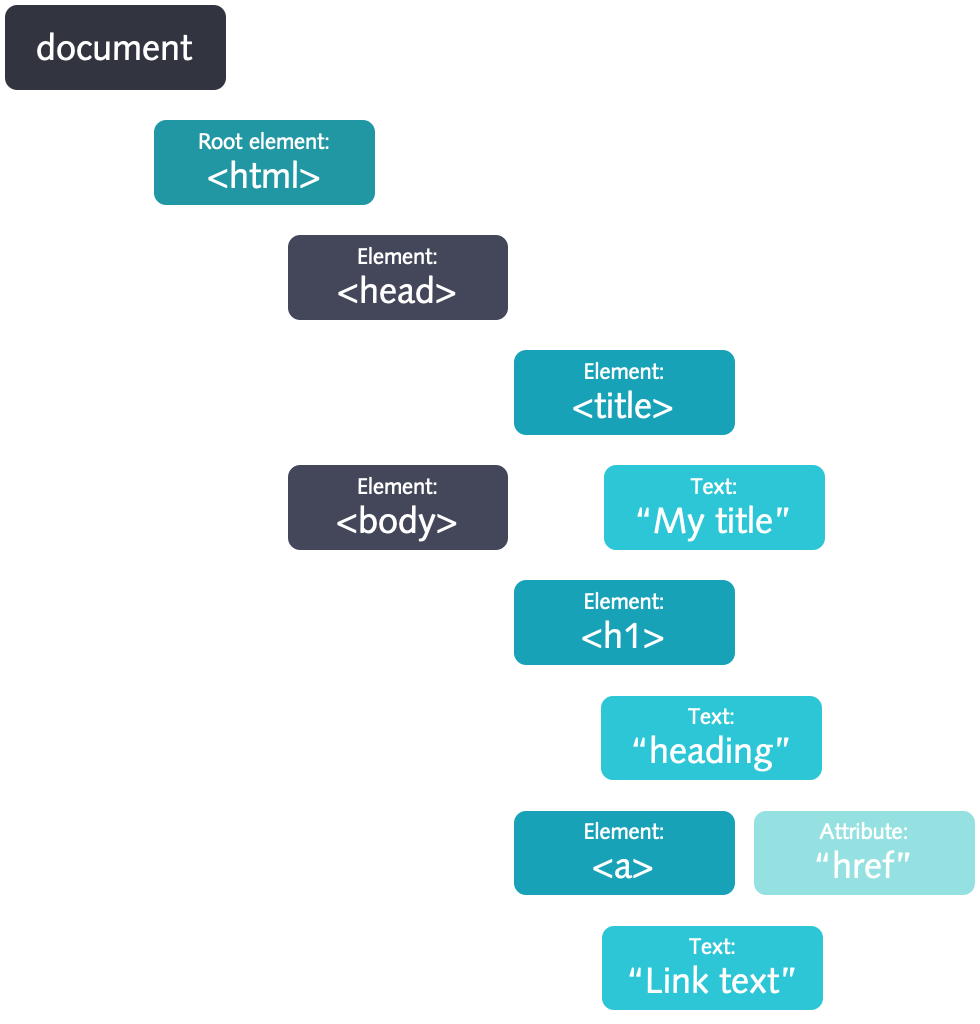
This is important to recognize, because it allows tags to be nested within each other. The <body> and <head> tags are nested within <html>, and <p> is nested within <body>. This nesting gives HTML a “tree-like” structure called Document Object Model (DOM). If a tag has other tags nested within it, we would refer to the containing tag as the parent and each of the tags within it as the “children”. If there is more than one child in a parent, the child tags are collectively referred to as “siblings”. These notions of parent, child and siblings give us an idea of the hierarchy of the tags. Each branch of this tree ends in a node and each node contains objects containing information. This structure allows programmatic access to the tree to change the structure, style or content of a document. We can use this DOM parsing to extract content of a website.
CSS
Whereas HTML provides the content and structure of a web page, CSS provides information about how a web page should be styled. Without CSS, a web page is dreadfully plain. When we say styling, we are referring to a wide, wide range of things. Styling can refer to the color of particular HTML elements or their positioning. Like HTML, the scope of CSS material is so large that we can’t cover every possible concept in the language. If you’re interested, you can learn more here:
If you want to practice the use of CSS selectors, this is a good site do do it:
Two concepts we do need to learn before we delve into the R web scraping code are classes and ids.
Classes
First, let’s talk about classes. If we were making a website, there would often be times when we’d want similar elements of a website to look and positioned the same.
For example, we might want a number of items in a list to all appear in the same color, red. We could accomplish that by directly inserting some CSS that contains the color information into each line of text’s HTML tag, like so:
<p style=”color:red” >Text 1</p>
<p style=”color:red” >Text 2</p>
<p style=”color:red” >Text 3</p>
The style text indicates that we are trying to apply CSS to the <p> tags. Inside the quotes, we see a key-value pair color:red. color refers to the color of the text in the <p> tags, while red describes what the color should be. But as we can see above, we’ve repeated this key-value pair multiple times. That’s not ideal — if we wanted to change the color of that text, we’d have to change each line one by one. Instead of repeating this style text in all of these <p> tags, we can replace it with a class selector:
<p class=”red-text” >Text 1</p>
<p class=”red-text” >Text 2</p>
<p class=”red-text” >Text 3</p>
With the class selector, we can better indicate that these <p> tags are related in some way. In a separate CSS file, we can creat the red-text class and define how it looks by writing:
.red-text {
    color: red;
}
Combining these two elements into a single web page will produce the same effect as the first set of red <p> tags, but it allows us to make quick changes more easily.
In this session, of course, we’re interested in web scraping, not building a web page (even though you can use that information to style your github page as well). But when we’re web scraping, we’ll often need to select a specific class of HTML tags, so we need understand the basics of how CSS classes work. Notice, that nodes can have multiple classes (separated by spaces).
Ids
Similarly, we may often want to scrape specific data that’s identified using an id. CSS ids are used to give a single element an identifiable name, much like how a class helps define a class of elements.
<p id=”special” >This is a special tag.</p>Don’t worry if you don’t quite understand classes and ids yet, it’ll become more clear when we start manipulating the code. You just need to know the following CSS Selector patterns used to select the styled elements.
Besides CSS selectors, you can also use Xpath (a XML path language) for selecting the nodes. Locating elements with XPath works very well with a little bit of more flexibility than CSS selectors. But most expressions can be directly translated from one to the other and vice versa.
| Goal | CSS | XPath |
|---|---|---|
| All Elements | * | //* |
| All P Elements | p | //p |
| All Child Elements | p > * | //p/* |
| Element By ID | #foo | //*[@id='foo’] |
| Element By Class | .foo | //*[contains(@class,‘foo’)] |
| Element With Attribute | *[title] | //*[@title] |
| First Child of All P | p > *first-child | //p/*[0] |
| All P with an A child | not possible | //p[a] |
| Next Element | p + * | //p/following-sibling::*[0] |
| Previous Element | not possible | //p/preceding-sibling::*[0] |
Selector gadget
A helpful tool to get the CSS Selector / xpath paths is the selectorgadget. It is a script that you can run on every website. You just have to click on the elements you want to select and it tells you the CSS / xpath code you need. Just add the following code to your bookmark bar, then go to any page and launch it.
javascript:(function()%7Bvar%20s=document.createElement('div');s.innerHTML='Loading...';s.style.color='black';s.style.padding='20px';s.style.position='fixed';s.style.zIndex='9999';s.style.fontSize='3.0em';s.style.border='2px%20solid%20black';s.style.right='40px';s.style.top='40px';s.setAttribute('class','selector_gadget_loading');s.style.background='white';document.body.appendChild(s);s=document.createElement('script');s.setAttribute('type','text/javascript');s.setAttribute('src','https://dv0akt2986vzh.cloudfront.net/unstable/lib/selectorgadget.js');document.body.appendChild(s);%7D)();But keep in mind, that there are infinite ways to select an element and having knowledge about the underlying html code of a website makes it way easier to scrape a website in the long run. To find the CSS class for an element, we need to right-click on that area and select “Inspect” or “Inspect Element” (depending on the browser you are using). The hardest part of scraping is figuring out the xpath or css to indicate which html nodes to select.
There are several R libraries designed to take HTML and the CSS selectors of the webpage for finding the relevant fields which contain the desired information. The library we’ll use in this tutorial is rvest. This package contains the basic web scraping functions, which are quite effective. Using the following functions, we will try to extract the data from web sites:
read_html(url): scrape entire HTML content from a given URLhtml_nodes(css = ".class""): calls node based on CSS classhtml_nodes(css = "#id""): calls node based on idhtml_nodes(xpath = "xpath"): calls node based on the given xpathhtml_attrs(): identifies attributeshtml_text(): strips the HTML tags and extracts only the texthtml_table(): turns HTML tables into data frames
The package stringr comes into play when you think of tasks related to data cleaning and preparation. stringr functions are useful because they enable you to work around the individual characters within the strings in character vectors.
str_detect(x, pattern)tells you if there’s any match to the pattern.str_count(x, pattern)counts the number of patterns.str_subset(x, pattern)extracts the matching components.str_locate(x, pattern)gives the position of the match.str_extract(x, pattern)extracts the text of the match.str_match(x, pattern)extracts parts of the match defined by parentheses.str_replace(x, pattern, replacement)/str_replace_all(x, pattern, replacement)replaces the matches with new text.#str_split(x, pattern)splits up a string into multiple pieces.
These pattern matching functions recognize four parts of pattern description. Regular expressions (RegEx) are the standard:
RegEx
| Category | RegEx | Explanation | Online example |
|---|---|---|---|
| Anchors | ^The | matches any string that starts with The | Try it! |
| Anchors | end$ | matches any string that ends with end | Try it! |
| Anchors | ^The end$ | exact string match (starts and ends with The end) | — |
| Quantifiers | abc* | matches a string that has ab followed by zero or more c | — |
| Quantifiers | abc+ | matches a string that has ab followed by one or more c | — |
| Quantifiers | abc? | matches a string that has ab followed by zero or one c | — |
| Quantifiers | abc{n} | matches a string that has ab followed by exact n c | — |
| Quantifiers | abc{n,} | matches a string that has ab followed by n or more c | — |
| Quantifiers | abc{n,m} | matches a string that has ab followed by n up to m c | — |
| Quantifiers | a(bc)* | matches a string that has a followed by zero or more copies of the sequence bc | — |
| Quantifiers | a(bc){n,m} | matches a string that has a followed by n up to m copies of the sequence bc | — |
| OR Operator | a(b|c) | matches a string that has a followed by b or c (and captures b or c) | — |
| OR Operator | a[bc] | same as previous, but without capturing b or c | — |
| Character classes | \d (negated \D) | matches a single character that is a digit | — |
| Character classes | \w (negated \W) or [:space:] | matches a word character (alphanumeric character plus underscore) | — |
| Character classes | \s (negated \S) | matches a whitespace character | — |
| Character classes | . | matches any character | — |
| Bracket expressions | [abc] or [a-c] | matches a string that has either an a or a b or a c | — |
| Bracket expressions | [a-fA-F0-9] or [:xdigit:] | a string that represents a single hexadecimal digit, case insensitively | — |
| Bracket expressions | [0-9] or [:digit:] | a string that has a character from 0 to 9 | — |
| Bracket expressions | [:alpha:] | Alphabetic characters: [:lower:] and [:upper:] | — |
| Bracket expressions | [:alnum:] | AAlphanumeric characters: [:alpha:] and [:digit:] | — |
| Bracket expressions | [^a-zA-Z] | a string that has not a letter from a to z or from A to Z. In this case the ^ is used as negation of the expression | — |
In order to be taken literally, you must escape the characters ^.[$()|*+?{\ with a backslash \ as they have special meaning. Notice that you can match also non-printable characters like tabs \t, new-lines \n, carriage returns \r.
Greedy and Lazy match
By default repetition of the quantifiers (*,+ and {}) is greedy, so the maximal possible number of repeats is used. For example, <.+> matches <div>simple div</div> in This is a <div> simple div</div> test.
In order to catch only the opening div tag we can append a ? to the quantifier to make it lazy: <.+?> will match <div> in this example.
Look-ahead and Look-behind — (?=) and (?<=)
| Category | RegEx | Explanation | Online example |
|---|---|---|---|
| Look-ahead | d(?=r) | matches a d only if is followed by r, but r will not be part of the overall regex | Try it! |
| Look-behind | (?<=r)d | matches a d only if is preceded by an r, but r will not be part of the overall regex match | Try it! |
| Look-ahead | d(?!r) | matches a d only if is not followed by r, but r will not be part of the overall regex match | Try it! |
| Look-behind | (?<!r)d | matches a d only if is not preceded by an r, but r will not be part of the overall regex match | Try it! |
A combination of look-ahead and look-behind is a good way to extract something between two patterns.
Examples
1st example: Get all companies from the S&P 500 (wikipedia)
- assign the wikipedia URL to a variable
- read in the html from the URL
- Select the correct html nodes and extract the html table
In order to start parsing through a web page, we first need to request that data from the computer server that contains it. In rvest, the function that serves this purpose is the read_html() function. It takes in a web URL as an argument and returns a list object that contains the tree-like structure we discussed earlier.
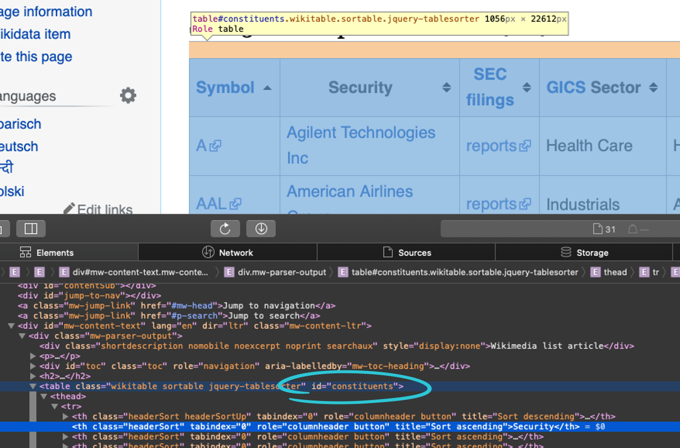
In order to capture the text, we need to use the html_nodes() and html_text() / html_table() functions respectively to search for this #constituents id and retrieve the text. Since we’re working with the tidyverse, we can just pipe the steps into the different functions. The code below does this:
# get the URL for the wikipedia page with all S&P 500 symbols
url <- "https://en.wikipedia.org/wiki/List_of_S%26P_500_companies"
# use that URL to scrape the S&P 500 table using rvest
library(rvest)
sp_500 <- url %>%
          # read the HTML from the webpage
          read_html() %>%
          # Get the nodes with the id
          html_nodes(css = "#constituents") %>%
          # html_nodes(xpath = "//*[@id='constituents']"") %>%
          # Extract the table and turn the list into a tibble
          html_table() %>%
          .[[1]] %>%
          as_tibble()
These functions together form the bulk of many common web scraping tasks. In general, web scraping in R (or in any other language) boils down to the following three steps:
- Get the HTML for the web page that you want to scrape
- Decide what part of the page you want to read and find out what HTML/CSS you need to select it
- Select the HTML and analyze it in the way you need
2nd example: Get the 250 top rated movies from IMDB
url  <- "https://www.imdb.com/chart/top/?ref_=nv_mv_250"
html <- url %>%
          read_html()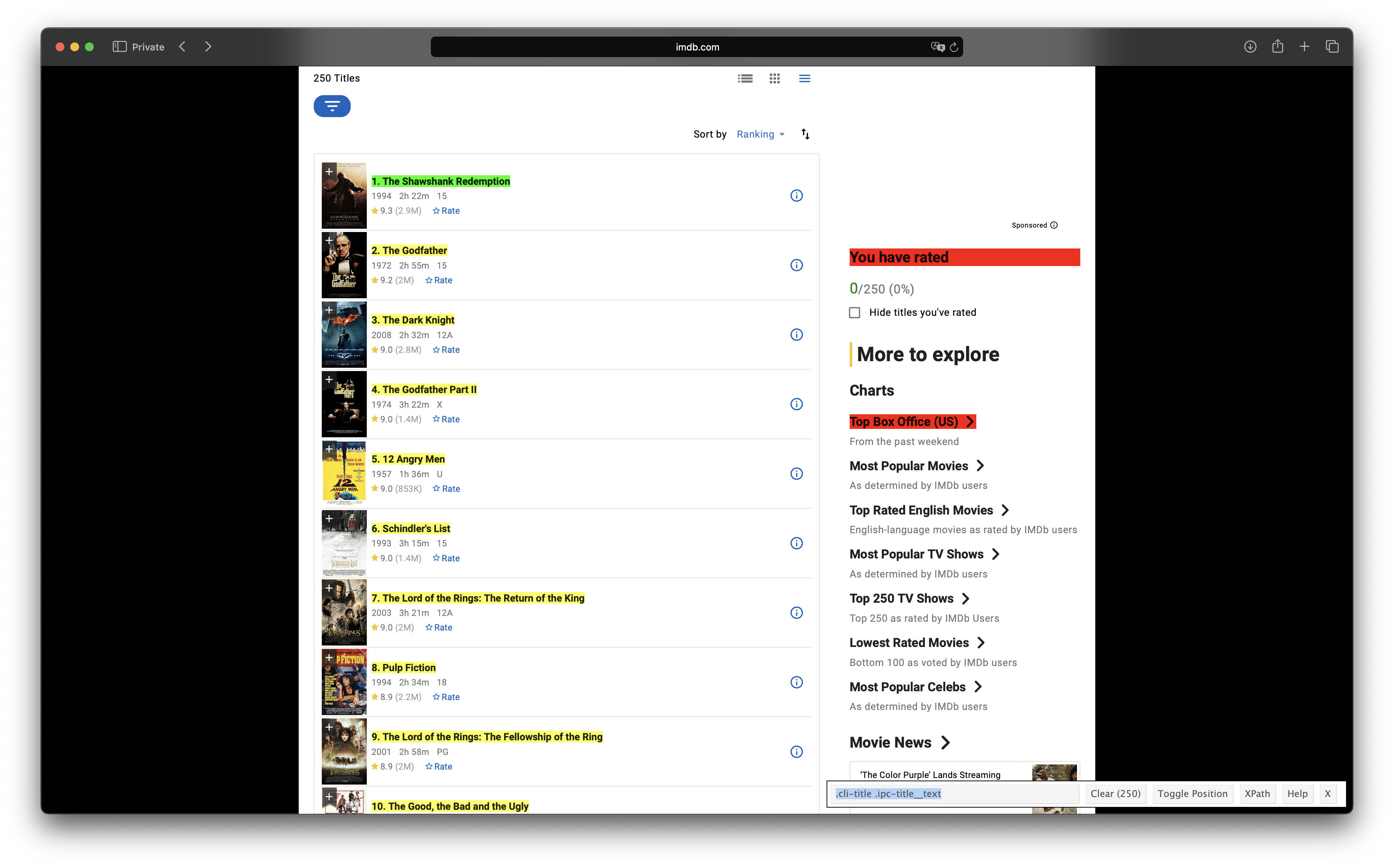
Get the ranks:
rank <- html |>
            html_elements(css = ".cli-title .ipc-title__text") |>
            html_text() |>
            parse_number()
Get the title: The title is in the child node with an a tag:
title <- html %>%
          html_elements(css = ".cli-title .ipc-title__text") |>
          html_text() |>
          str_remove("^\\d*\\. ") # Remove numbers, dot and space at the beginning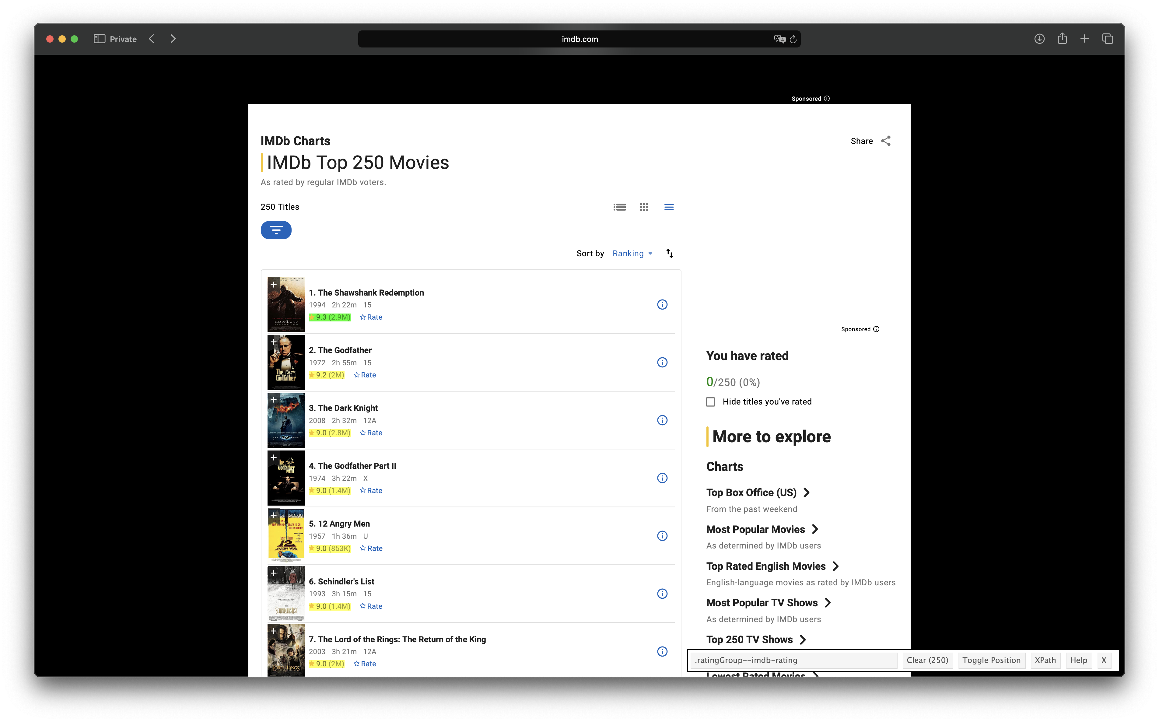
Get the ratings:
rating <- html %>%
  html_elements(css = ".ratingGroup--imdb-rating") |>
  html_text() |>
  str_remove("\\(.*\\)") |>
  str_squish() |>
  as.numeric()
Merge everything into a tibble:
imdb_tbl <- tibble(rank, title, rating)

imdb_tbl
## # A tibble: 250 × 3
##     rank title                                       rating
##
##  1     1 Die Verurteilten                               9.3
##  2     2 Der Pate                                       9.2
##  3     3 The Dark Knight                                9
##  4     4 Der Pate 2                                     9
##  5     5 Die zwölf Geschworenen                         9
##  6     6 Schindlers Liste                               9
##  7     7 Der Herr der Ringe: Die Rückkehr des Königs    9
##  8     8 Pulp Fiction                                   8.9
##  9     9 Der Herr der Ringe: Die Gefährten              8.9
## 10    10 Zwei glorreiche Halunken                       8.8
## # ℹ 240 more rows
## # ℹ Use `print(n = ...)` to see more rows
As a side note, if you run the code from a country where English is not the main language, it’s very likely that you’ll get some of the movie names translated into the main language of that country.
Most likely, this happens because the server infers your location from your IP address.
If you run into this issue, retrieve the html content with the GET() function from the httr package and pass the following values to the headers parameter:
resp <- GET(url = "https://www.imdb.com/chart/top/?ref_=nv_mv_250",
            add_headers('Accept-Language' = "en-US, en;q=0.5"))
html <- content(resp)
This will communicate the server something like “I want the linguistic content in American English (en-US). If en-US is not available, then other types of English (en) would be fine too (but not as much as en-US)”. The q parameter indicates the degree to which we prefer a certain language (in this case we will accept other English languages if its translation quality is > 50 %). If not specified, then the values is set to 1 by default, like in the case of en-US. You can read more about this here.
Functional programming
If we scrape more than one page, we usually have to iterate over the content. Iterating refers to programmatically repeating a step or sets of steps, a set number of times or until a condition is met.
Typically, when we iterate in any programming language, we use a loop, typically a for loop:
for (variable in vector) {

}
# Example: For Loop
numbers <- c(1:5)
for (i in numbers) {
   print(i)
}
## 1
## 2
## 3
## 4
## 5
Almost every iteration can be done with a for loop, but using the purrr package is a better idea. Loops in R are slow and hard to read. The purrr package provides a suite of functions for iteration and functional programming that integrate well with the rest of the tidyverse. The core function in purrr is map(), that serves to apply a function to all elements of an object. The base R function of map() is lapply() (and its variants sapply(), vapply(), …), which does almost the same. But if we work in the tidyverse, map() is rather useful.
The above for loop would be written like this:
# purr functional programming approach
numbers_list <- map(numbers, print)
## 1
## 2
## 3
## 4
## 5
A few things to note:
- both the for loop and map function do an operation for each element in the vector
- the map function returns a nested list where each entry is the result of the function called inside of it for one of the entries in the object that being iterated over. Assign this to a variable to avoid it from printing.
- Using purrr’s map function is only one line and less code
- Using purrr’s map function is easier to read
Another useful function from the purrr package is pluck(). It makes it easy to extract certain elements from lists, which is particularly helpful, if we want to extract data from json files.
Let’s take a look at the following json file (you will see in the business case where it comes from). Download it to your computer and read it into R with the jsonlite package.
bike_data_lst <- fromJSON("bike_data.json")
# Open the data by clicking on it in the environment or by running View()
View(bike_data_lst)
There we can navigate through the list by clicking on the blue arrows. This json contains data about bikes listed on a website. Let’s try to find the different color variations of the bike. This is the path:
productDetail --> variationAttributes --> values --> [[1]] --> displayValueIf we go to the right side of the viewer, a button appears. Clicking it will send the code to the console, that extract exactly those values.
bike_data_lst[["productDetail"]][["variationAttributes"]][["values"]][[1]][["displayValue"]]
## "Stealth"     "aero silver"
pluck() does exactly the same, but looks rather neat. You just have to separate the path by commas:
bike_data_lst %>%
  purrr::pluck("productDetail", "variationAttributes", "values", 1, "displayValue")
## "Stealth"     "aero silver"
Business Case
Goal
There are many use cases: Contact Scraping, Monitoring/Comparing Prices, Scraping Reviews/Ratings etc.
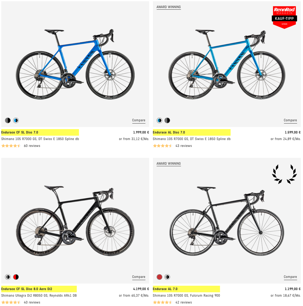
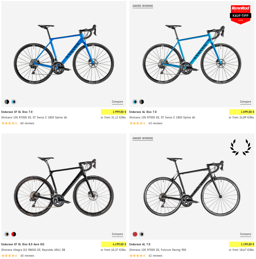
In this case you learn how to web-scrape all bike models from the bike manufacturer Canyon to put into a strategic database with competitor product data. The individual product pages have a ton of valuable information. Hence, we have to find a way to get all individual product URLs to scrape the content for our strategic database.
The following steps describe how you get the bike data, which you have already used in the last session.
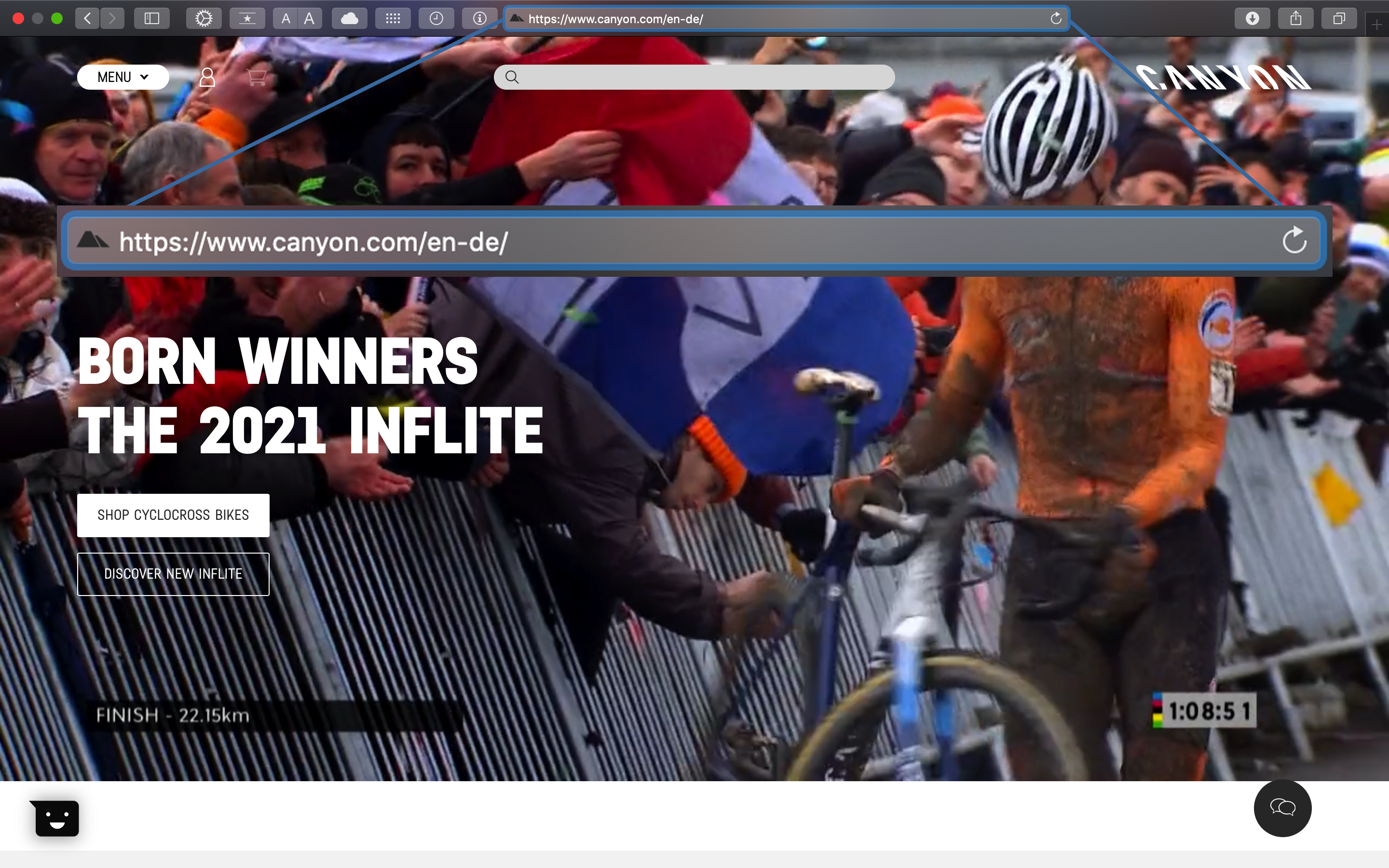
The starting point is the analysis of the URL, website and product structure of your competitor. The URL consists of a base path and several page paths:
- URL Base path / Landing page / Home
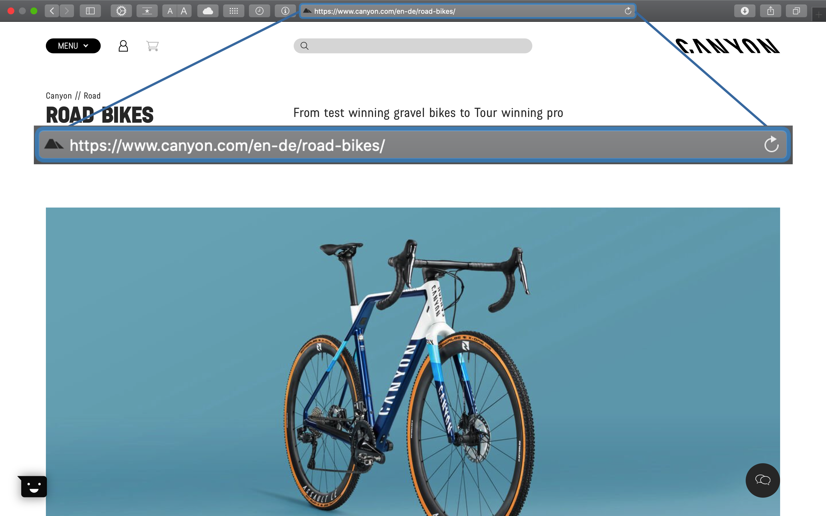
The products are divided into FAMILIES and CATEGORIES:
URL Page path for the product FAMILIES:
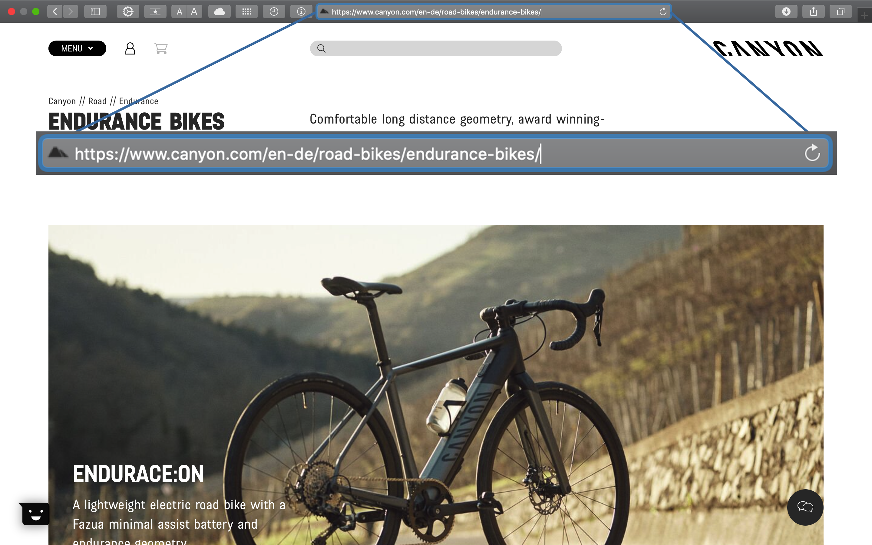
URL Page path for the product CATEGORIES (the ride styles,
endurance-bikesin this example, don’t matter to us):
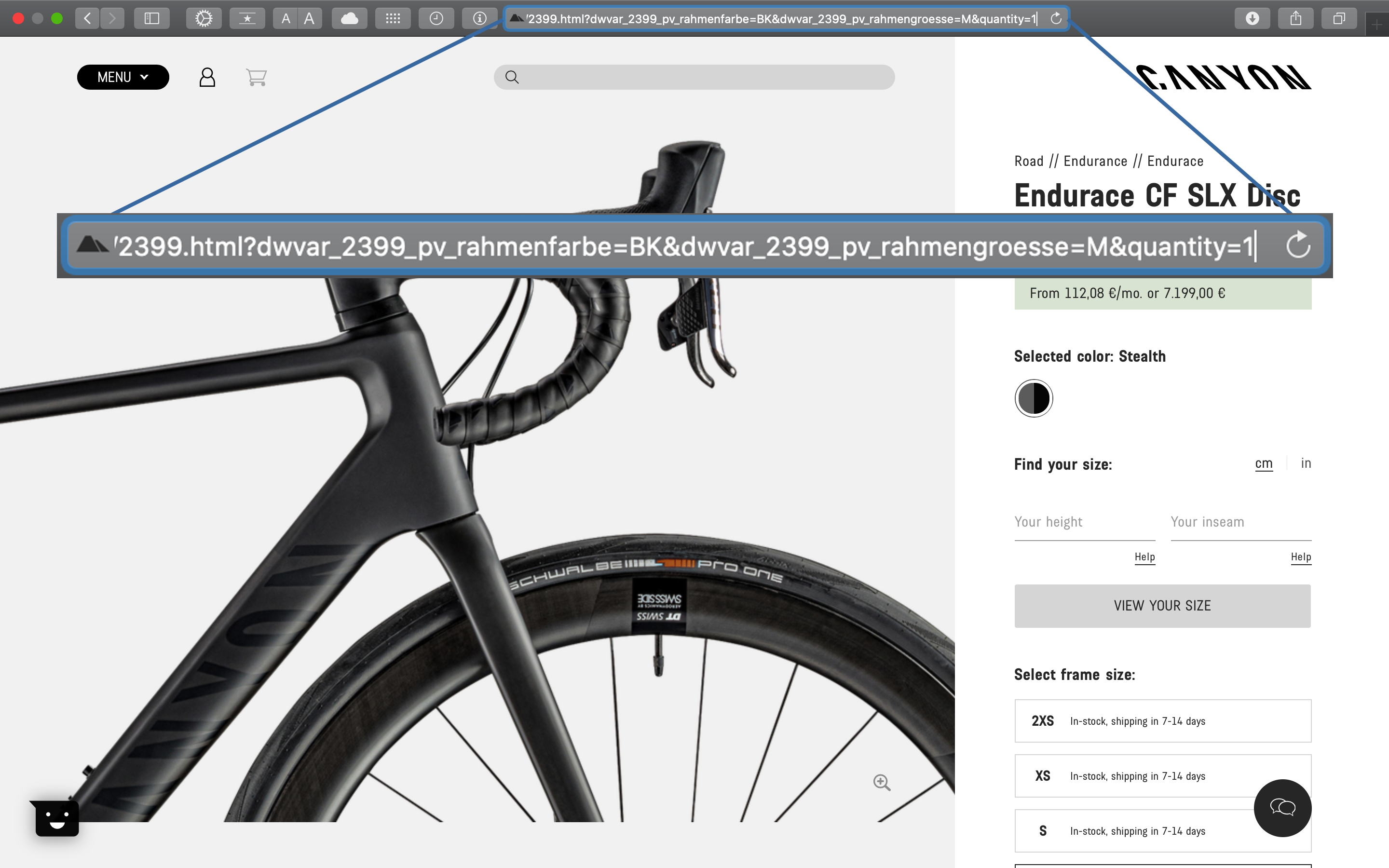
Each bike can come in different color variations (indicated by ?dwvar_2399_pv_rahmenfarbe=BK in this example)
- URL query parameters (initialized by the question mark
?)
Our goal is to get the current prices for every bike model. We can do that, if we are able to retrieve the PRODUCT URLs for each individual bike model (It is also possible to create the URLs for each color scheme. But focusing solely on the model is sufficient for now).
Analysis with R
First, we have to load the relevant libraries.
# WEBSCRAPING ----

# 1.0 LIBRARIES ----
library(tidyverse) # Main Package - Loads dplyr, purrr, etc.
library(rvest)     # HTML Hacking & Web Scraping
library(xopen)     # Quickly opening URLs
Page analysis
Analyze the page to make a plan for our web scraping approach (there is no unique way. Possibly there are hundreds of ways to get that data.)
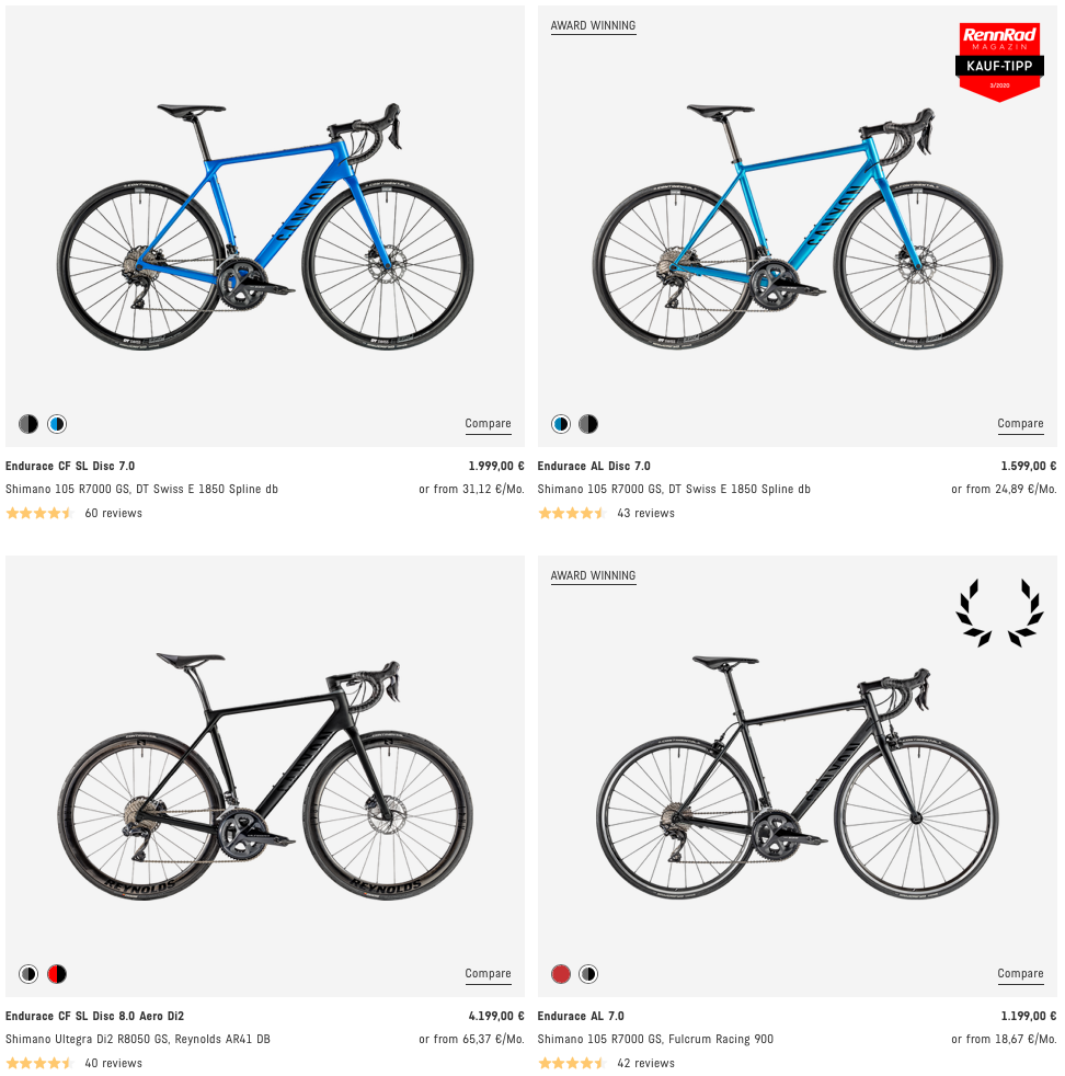
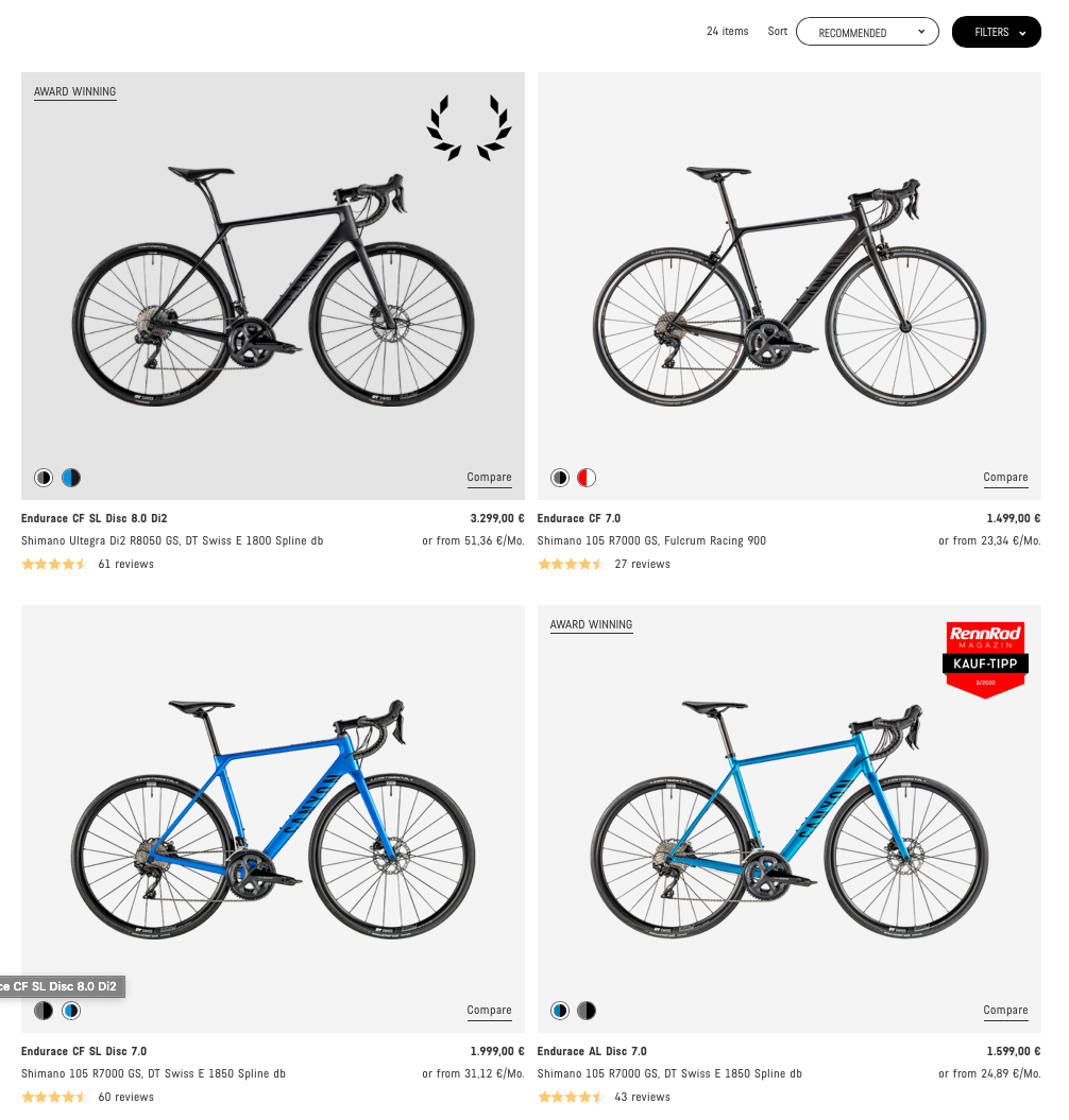
- Where are the individual bikes listed, so that we can scrape their URLs? –> On the product CATEGORY sites (e.g. https://www.canyon.com/en-de/road-bikes/endurance-bikes/endurace/):
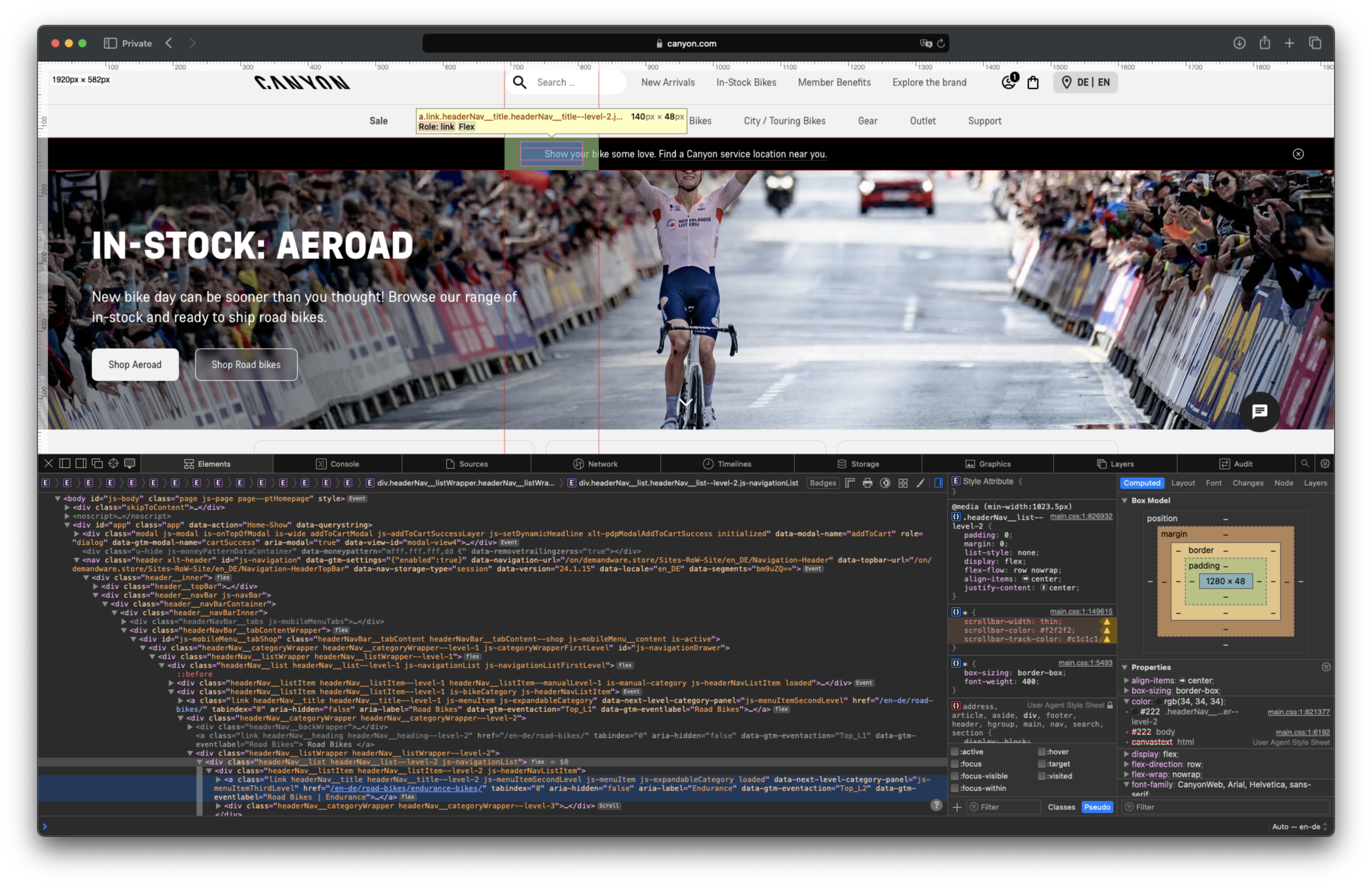
- Where can we find all product category sites? –> If we hover over a product family in the navigation bar (e.g. Road Bikes), always one level below (e.g. Endurance, Race, …). The bar is not shown in the screenshot below because the cursor was hovering over the corresponding HTML node at the bottom.
Scraping
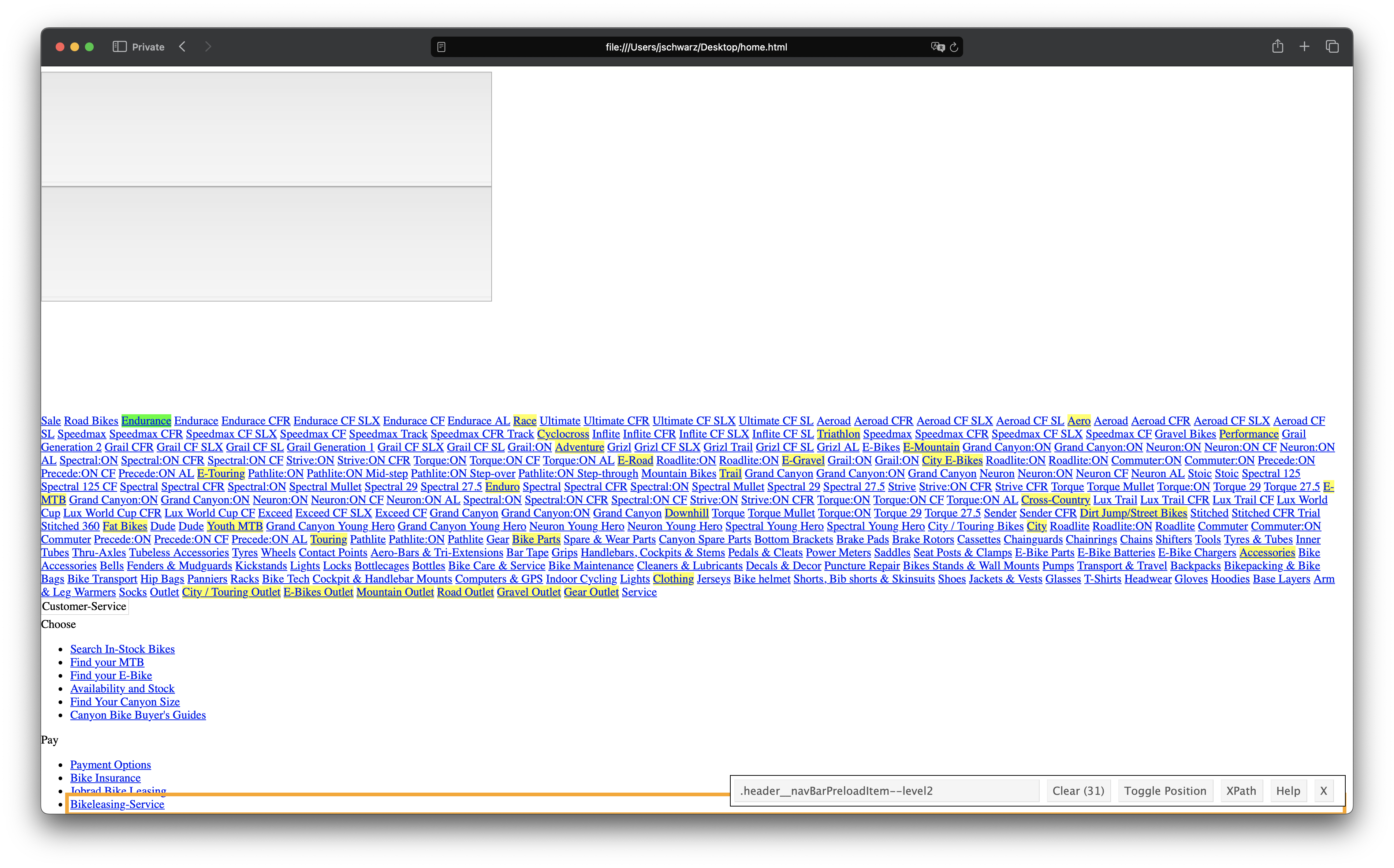
Inspecting the file manually first makes sense, because R retrieves the page in a different way than we do inside a browser:
html_home <- read_html(url_home)
html_home |> xml2::write_html("home.html")
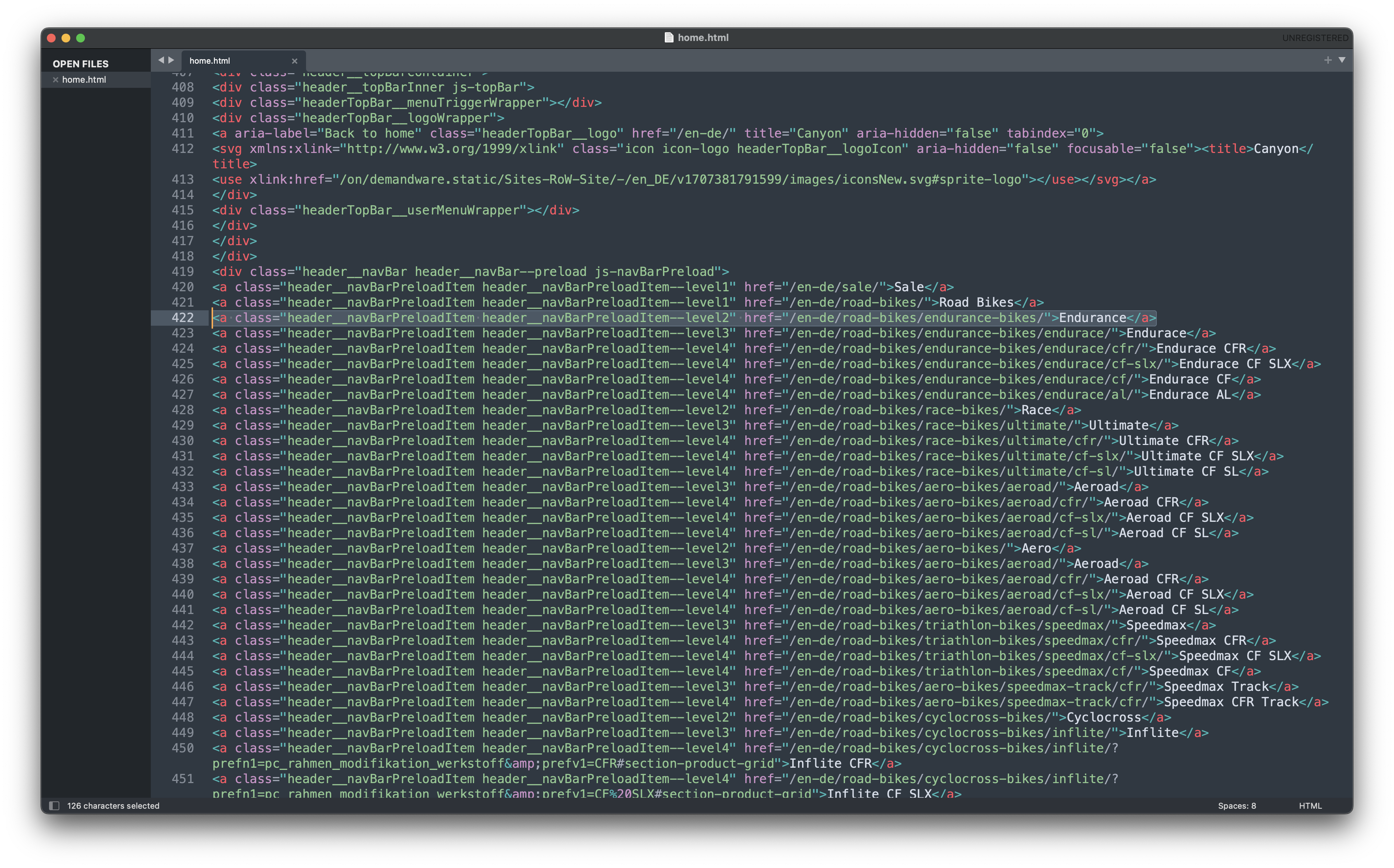
Step 1: Get URLs for each of the product CATEGORIES
# 1.2 COLLECT PRODUCT CATEGORIES ----

url_home        <- "https://www.canyon.com/en-de"
xopen(url_home) # Open links directly from RStudio to inspect them

# Read HTML for the entire webpage
html_home       <- read_html(url_home)

# Extract the categories URLs (Roadbike-Endurance, Roadbike-Race, ...)
# All Models are listed on these levels.
bike_categories_chr <- html_home |>

  # Get the nodes for the categories. Take a look at the source code for the selector.
  # (Unfortunately not working with the Selector Gadget with the original page)
  html_elements(css = ".header__navBarPreloadItem--level2") |>

  # Extract the href attribute (the URLs)
  html_attr('href') |>

  # Remove the product families Sale, Outlet, Gear and Customer Service
  str_subset(pattern = "sale|outlet|gear|customer-service", negate = T) |>

  # Add the domain, because we will get only the subdirectories
  # Watch out for the new pipe placeholder `_` here.
  # It requires a named argument (`...` in this case)
  str_c("https://www.canyon.com", ... = _)

bike_categories_chr
##  [1] "https://www.canyon.com/en-de/road-bikes/endurance-bikes/"             "https://www.canyon.com/en-de/road-bikes/race-bikes/"
##  [3] "https://www.canyon.com/en-de/road-bikes/aero-bikes/"                  "https://www.canyon.com/en-de/road-bikes/cyclocross-bikes/"
##  [5] "https://www.canyon.com/en-de/road-bikes/triathlon-bikes/"             "https://www.canyon.com/en-de/gravel-bikes/performance/"
##  [7] "https://www.canyon.com/en-de/gravel-bikes/adventure/"                 "https://www.canyon.com/en-de/electric-bikes/electric-mountain-bikes/"
##  [9] "https://www.canyon.com/en-de/electric-bikes/electric-road-bikes/"     "https://www.canyon.com/en-de/electric-bikes/electric-gravel-bikes/"
## [11] "https://www.canyon.com/en-de/electric-bikes/electric-city-bike/"      "https://www.canyon.com/en-de/electric-bikes/electric-touring-bikes/"
## [13] "https://www.canyon.com/en-de/mountain-bikes/trail-bikes/"             "https://www.canyon.com/en-de/mountain-bikes/enduro-bikes/"
## [15] "https://www.canyon.com/en-de/electric-bikes/electric-mountain-bikes/" "https://www.canyon.com/en-de/mountain-bikes/cross-country-bikes/"
## [17] "https://www.canyon.com/en-de/mountain-bikes/downhill-bikes/"          "https://www.canyon.com/en-de/mountain-bikes/dirt-jump-bikes/"
## [19] "https://www.canyon.com/en-de/mountain-bikes/fat-bikes/"               "https://www.canyon.com/en-de/mountain-bikes/youth-kids/"
## [21] "https://www.canyon.com/en-de/hybrid-bikes/city-bikes/"                "https://www.canyon.com/en-de/hybrid-bikes/touring-bikes/"
Step 2: Get the URLs for each individual bike for each product category. You might have to scroll down a bit (depending on the category).
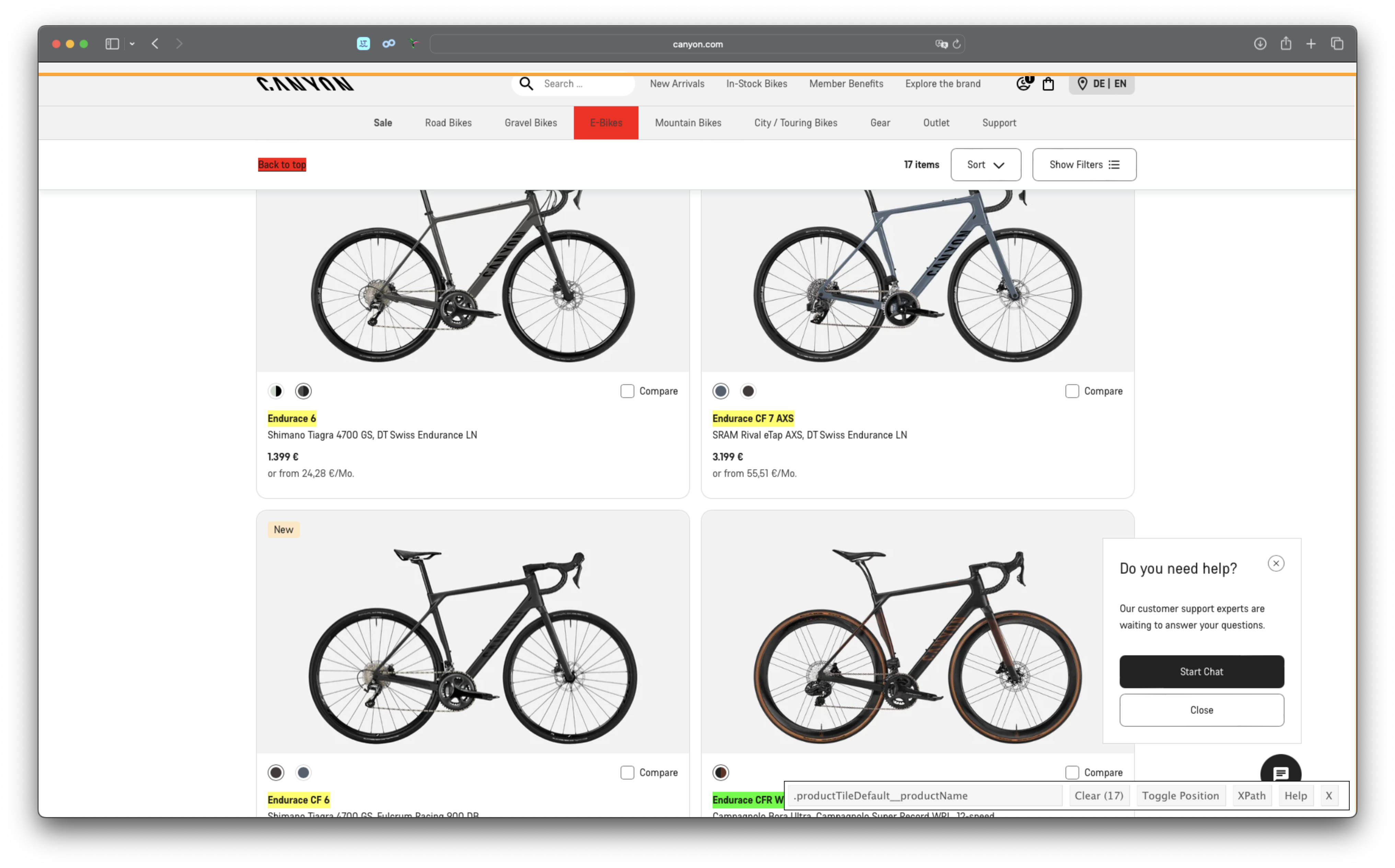
Step 2.1: Test it for one category
# 2.0 COLLECT BIKE DATA ----

# Select first bike category url
bike_category_url <- bike_categories_chr[1]

# Get the URLs for the bikes of the first category
html_bike_category  <- read_html(bike_category_url)

bike_url_chr        <- html_bike_category |>

                          # Get the 'a' nodes that containt the title and the link
                          html_elements(".productTileDefault__productName") |>

                          # html_elements(css = ".productTileDefault--bike > div > a") |>
                          html_attr("href") |>

                          # Remove the query parameters of the URL (everything after the '?')
                          str_remove(pattern = "\\?.*")

bike_url_chr
## [1] "https://www.canyon.com/en-de/road-bikes/endurance-bikes/endurace/al/endurace-6/3718.html"
## [2] "https://www.canyon.com/en-de/road-bikes/endurance-bikes/endurace/cf/endurace-cf-7-axs/3708.html"
## [3] "https://www.canyon.com/en-de/road-bikes/endurance-bikes/endurace/cf/endurace-cf-6/3706.html"
## [4] "https://www.canyon.com/en-de/road-bikes/endurance-bikes/endurace/cfr/endurace-cfr-wrl/3490.html"
## [5] "https://www.canyon.com/en-de/road-bikes/endurance-bikes/endurace/cf/endurace-cf-7/3707.html"
Step 2.2: Make a function to get the bike model urls for each category (just wrap the above code into the function() function)
# 2.2 Wrap it into a function ----
get_bike_urls <- function(url) {

  html_bike_category <- read_html(url)

  # Get the URLs
  bike_url_chr  <- html_bike_category |>
    html_elements(css = ".productTileDefault__productName") |>
    html_attr("href") |>
    str_remove(pattern = "\\?.*")

  return(bike_url_chr)

}

# Run the function with the first url to check if it is working
get_bike_urls(url = bike_categories_chr[1])

# Map the function against all urls
bike_urls_chr <- map(bike_categories_chr, get_bike_urls) |>
                      flatten_chr() |>
unique()- Step 3: Get the model names and prices. You don’t need to do it for all. We can subset the data beforehand.
3.1: Subsetting:
# Split data to enable filtering
bike_urls_tbl <- bike_urls_chr |>

  tibble::as_tibble_col(column_name = "url") |>
  tidyr::separate_wider_regex(cols = url, patterns = c(".*en-de/", family   = "[^/]*", "/",
                                                       category = "[^/]*", "/",
                                                       model    = "[^/]*", "/",
                                                       material = "[^/]*", "/",
                                                       ".*"), cols_remove = F)

# Filter
bike_urls_endurace_tbl <- bike_urls_tbl |>
  filter(model == "endurace")

# Print
bike_urls_endurace_tbl |> slice(1:5)
## # A tibble: 5 × 5
##   family     category        model    material url
##
## 1 road-bikes endurance-bikes endurace al       https://www.canyon.com/en-de/road-bikes/endurance-bikes/endurace/al/endurace-6/3718.html
## 2 road-bikes endurance-bikes endurace cf       https://www.canyon.com/en-de/road-bikes/endurance-bikes/endurace/cf/endurace-cf-7-axs/3708.html
## 3 road-bikes endurance-bikes endurace cf       https://www.canyon.com/en-de/road-bikes/endurance-bikes/endurace/cf/endurace-cf-6/3706.html
## 4 road-bikes endurance-bikes endurace cfr      https://www.canyon.com/en-de/road-bikes/endurance-bikes/endurace/cfr/endurace-cfr-wrl/3490.html
## 5 road-bikes endurance-bikes endurace cf       https://www.canyon.com/en-de/road-bikes/endurance-bikes/endurace/cf/endurace-cf-7/3707.html
3.2: Get name and prices for the endurace cateogory bikes
# For 1 bike
html_bike_model <- read_html(bike_urls_endurace_tbl$url[1])

bike_price <- html_bike_model |>
  html_element(css = ".productDescription__priceSale") |>
  html_text() |>
  parse_number() |>
  str_remove("\\.")

bike_model <- html_bike_model |>
  html_elements(css = ".xlt-pdpName") |>
  html_text() |>
  str_squish() # Clean

# Function to do it for multiple urls
get_model_data <- function(url) {

  html_bike_model <- read_html(url)

  bike_price <- html_bike_model |>
    html_element(css = ".productDescription__priceSale") |>
    html_text() |>
    parse_number() |>
    str_remove("\\.")

  bike_model <- html_bike_model |>
    html_elements(css = ".xlt-pdpName") |>
    html_text() |>
    str_squish() # Clean

  bike_data <- tibble(url   = url,
                      model = bike_model,
                      price = bike_price)

  return(bike_data)

}
Run Function
# For one model
bike_model_data_tbl <- get_model_data(url = bike_urls_endurace_tbl$url[1])

# For all models of the category
bike_model_data_tbl <- bike_urls_endurace_tbl$url |> map_dfr(get_model_data)

# Join data
bike_model_data_joined_tbl <- bike_urls_endurace_tbl |>
                                  left_join(bike_model_data_tbl, by = join_by("url"))

# Print
bike_model_data_joined_tbl
## # A tibble: 17 × 7
##    family     category        model.x  material url                                                                                                          model.y                    price
##
##  1 road-bikes endurance-bikes endurace al       https://www.canyon.com/en-de/road-bikes/endurance-bikes/endurace/al/endurace-6/3718.html                     Endurace 6                 1399
##  2 road-bikes endurance-bikes endurace cf       https://www.canyon.com/en-de/road-bikes/endurance-bikes/endurace/cf/endurace-cf-7-axs/3708.html              Endurace CF 7 AXS          3199
##  3 road-bikes endurance-bikes endurace cf       https://www.canyon.com/en-de/road-bikes/endurance-bikes/endurace/cf/endurace-cf-6/3706.html                  Endurace CF 6              1999
##  4 road-bikes endurance-bikes endurace cfr      https://www.canyon.com/en-de/road-bikes/endurance-bikes/endurace/cfr/endurace-cfr-wrl/3490.html              Endurace CFR WRL           8999
##  5 road-bikes endurance-bikes endurace cf       https://www.canyon.com/en-de/road-bikes/endurance-bikes/endurace/cf/endurace-cf-7/3707.html                  Endurace CF 7              2499
##  6 road-bikes endurance-bikes endurace al       https://www.canyon.com/en-de/road-bikes/endurance-bikes/endurace/al/endurace-7/3705.html                     Endurace 7                 1699
##  7 road-bikes endurance-bikes endurace cfr      https://www.canyon.com/en-de/road-bikes/endurance-bikes/endurace/cfr/endurace-cfr-di2/2742.html              Endurace CFR Di2           8999
##  8 road-bikes endurance-bikes endurace cf-slx   https://www.canyon.com/en-de/road-bikes/endurance-bikes/endurace/cf-slx/endurace-cf-slx-7-axs/3087.html      Endurace CF SLX 7 AXS      3999
##  9 road-bikes endurance-bikes endurace cf-slx   https://www.canyon.com/en-de/road-bikes/endurance-bikes/endurace/cf-slx/endurace-cf-slx-8-axs-aero/3712.html Endurace CF SLX 8 AXS Aero 5499
## 10 road-bikes endurance-bikes endurace cfr      https://www.canyon.com/en-de/road-bikes/endurance-bikes/endurace/cfr/endurace-cfr-axs/2743.html              Endurace CFR AXS           8499
## 11 road-bikes endurance-bikes endurace cf-slx   https://www.canyon.com/en-de/road-bikes/endurance-bikes/endurace/cf-slx/endurace-cf-slx-8-di2/3711.html      Endurace CF SLX 8 Di2      5199
## 12 road-bikes endurance-bikes endurace cf       https://www.canyon.com/en-de/road-bikes/endurance-bikes/endurace/cf/endurace-cf-8-di2/3709.html              Endurace CF 8 Di2          3799
## 13 road-bikes endurance-bikes endurace cf-slx   https://www.canyon.com/en-de/road-bikes/endurance-bikes/endurace/cf-slx/endurace-cf-slx-8-di2-aero/2740.html Endurace CF SLX 8 Di2 Aero 5199
## 14 road-bikes endurance-bikes endurace cf-slx   https://www.canyon.com/en-de/road-bikes/endurance-bikes/endurace/cf-slx/endurace-cf-slx-8-di2/2739.html      Endurace CF SLX 8 Di2      4199
## 15 road-bikes endurance-bikes endurace al       https://www.canyon.com/en-de/road-bikes/endurance-bikes/endurace/al/endurace-7-rb/2731.html                  Endurace 7 RB              1299
## 16 road-bikes endurance-bikes endurace al       https://www.canyon.com/en-de/road-bikes/endurance-bikes/endurace/al/endurace-7/2733.html                     Endurace 7                 1499
## 17 road-bikes endurance-bikes endurace cf       https://www.canyon.com/en-de/road-bikes/endurance-bikes/endurace/cf/endurace-cf-7/2735.html                  Endurace CF 7              1999
Further details
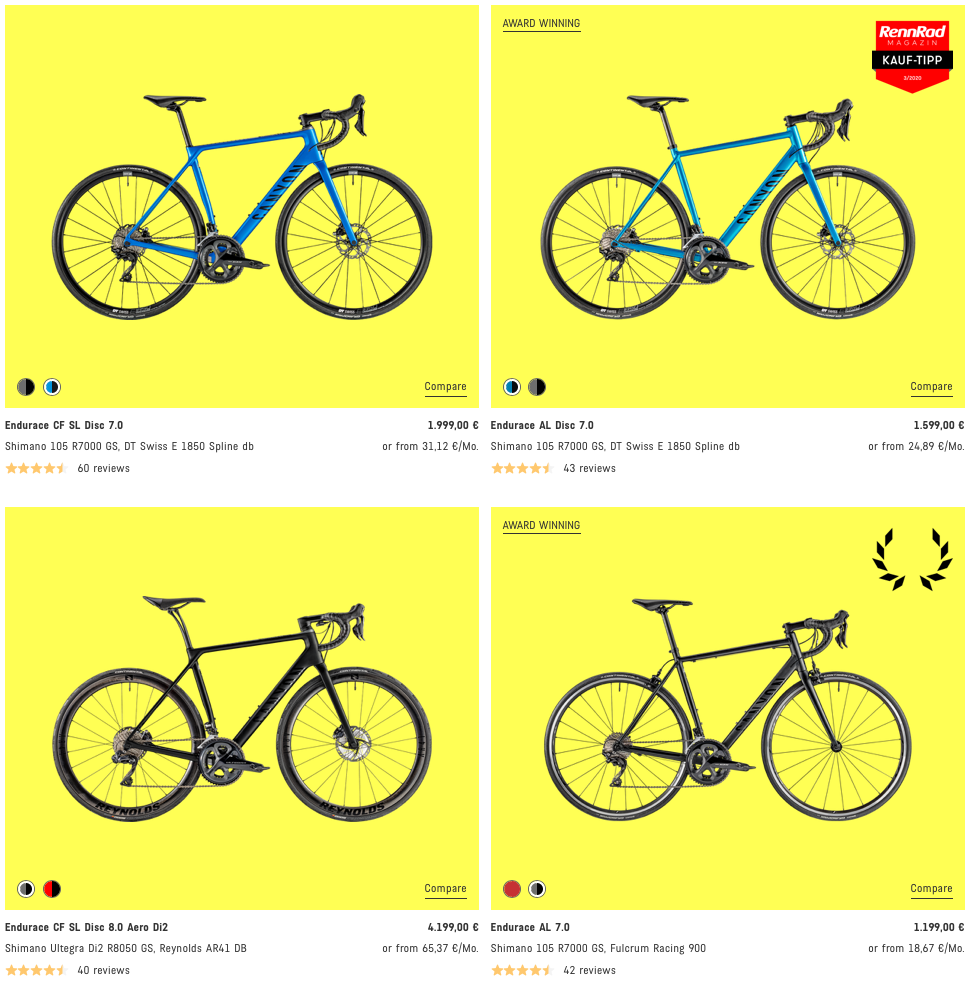
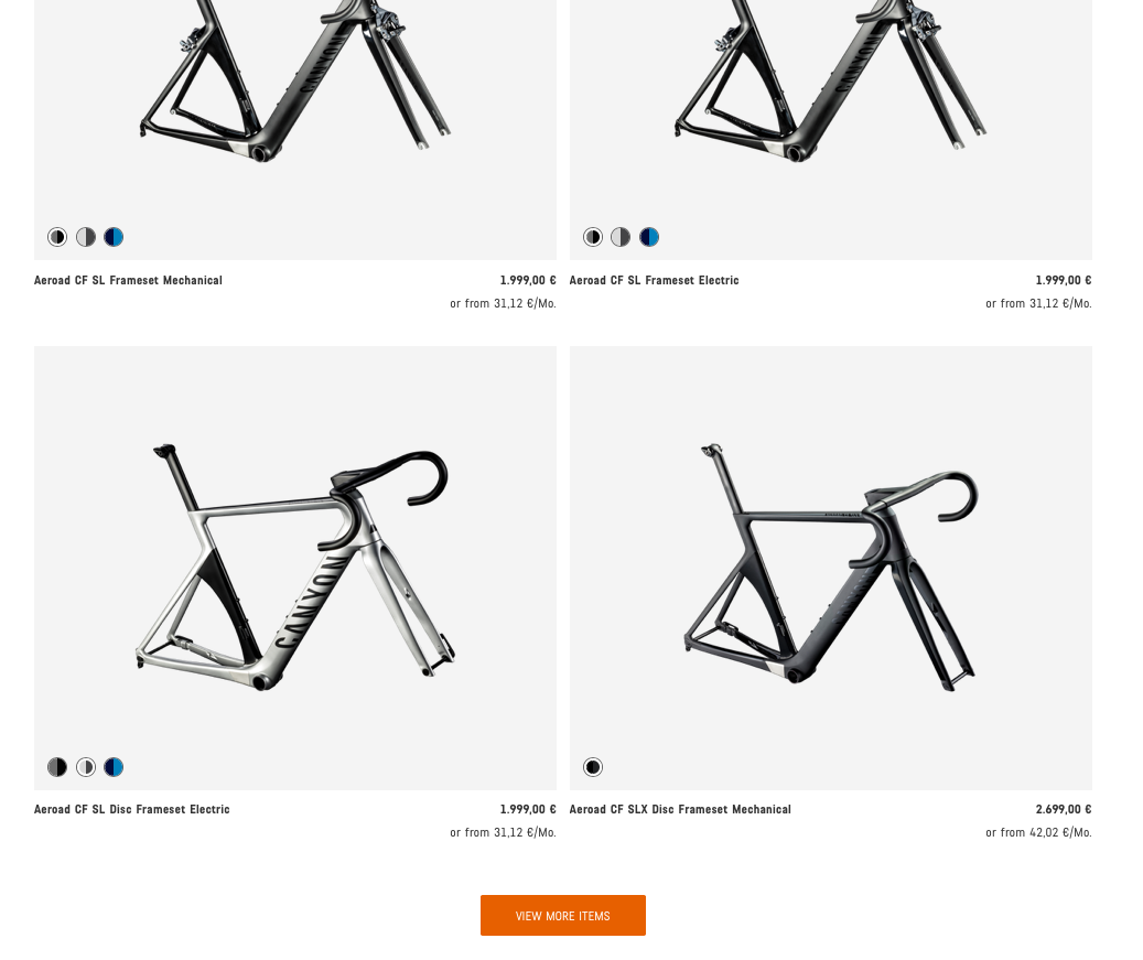
This was an introduction to web scraping static sites by using the library rvest. However, many web pages are dynamic and use JavaScript to load their content. These websites often require a different approach to gather the data. If you take a look at the following screenshot, you see, that also the website of Canyon uses JavaScript libraries like JQuery or ReactJs or Angular to dynamically create the HTML data. It will only be downloaded if we click the ‘View More Items’ button. So we can not simply use rvest to scrap the data if we want zo analyze the entire content (in this case only a few bikes/frames are not loaded).
To solve the problem, there is another solution. We can use the Selenium web scraping framework. Selenium automates browsers. Originally, it is developed to programmatically test websites. But using it we can also scrap data from websites. Selenium doesn’t have it’s own web browser. We need to integrate it into other web browsers in order to run. But we will use a web browser, which will be running in the background and controlled by our selenium library. And this type of browser is called, headless browser. A headless browser loads website into memory, executes JavaScript code on the page and everything happens in the background. Many web browsers like firefox and chrome support headless features.
Because I only want to mention this option and installing Selenium might be a little complicated, I am not going to explain the necessary steps in detail and provide you just the code how to click the button and get the entire html content.
library(RSelenium)
# Start the headless browser
driver <- rsDriver(browser = "firefox")
remDr  <- driver$client

# Open the url
url    <- "https://www.canyon.com/en-de/road-bikes/race-bikes/aeroad/"
remDr$navigate(url)

# Locate and click the button
button <- remDr$findElement(using = "css", ".productGrid__viewMore")
button$clickElement()

# Get the html
html <- remDr$getPageSource() %>%
              unlist() %>%
              read_html()
Things to keep in mind…
- Static & Well Structured: Web scraping is best suited for static & well structured web pages.
- Code Changes: The underling HTML code of a web page can change anytime due to changes in design or for updating details. In such case, your script will stop working. It is important to identify changes to the web page and modify the web scraping script accordingly.
- API Availability: In many cases, an API is made available by the service provider or organization. It is always advisable to use the API and avoid web scraping.
- IP Blocking: Do not flood websites with requests as you run the risk of getting blocked. Have some time gap between request so that your IP address is not blocked from accessing the website. Of course, you can also learn to work your way around the anti scraping methods. However, you do need to understand the legality of scraping data and whatever you are doing with the scraped data: http://www.prowebscraper.com/blog/six-compelling-facts-about-legality-of-web-scraping/
Datacamp
Challenge
In this chapter, there are two challenges for you:
Get some data via an API. There are millions of providers, that offer API access for free and have good documentation about how to query their service. You just have to google them. You can use whatever service you want. For example, you can get data about your listening history (spotify), get data about flights (skyscanner) or just check the weather forecast. Print the data in a readable format, e.g. a table if you want, you could also plot it.
Scrape one of the competitor websites of canyon (either https://www.rosebikes.de/ or https://www.radon-bikes.de) and create a small database. The database should contain the model names and prices for at least one category. Use the
selectorgadgetto get a good understanding of the website structure, it is really helpful. After scraping your data, convert it to a readable format. Prices should be in a numeric format without any other letters or symbols. Also check if the prices are reasonable.
Upload your codes to your github page. Print the first 10 rows of your tibbles. Keep in mind that you should not publish your credentials.