Introduction to R, RStudio IDE & GitHub
This chapter provides a broad overview of the R language that will get you programming right away. The first project will be creating a decision tool used in cost accounting. This project will make it easier to study these things by teaching you the basics of R. The term “R” is used to refer to both the programming language and the software that interprets the scripts written using it. Your first mission is simple: assemble R code that will calculate the ideal quantity of inventory to order for a given product (Economic Order Quantity).
In this project, you will learn how to:
- Use the R and RStudio interfaces
- Run R commands
- Create R objects
- Write your own R functions and scripts
Don’t worry if you’ve never programmed before and it seems like we cover a lot of ground fast. The chapter will teach you everything you need to know and gives you a concise overview of the R language. You will return to many of the concepts we meet here in the next projects, where you will examine the concepts in depth.
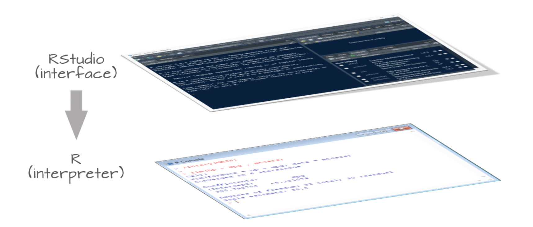
Before you can ask your computer to save some numbers, you’ll need to know how to talk to it. RStudio gives you a way to talk to your computer. R gives you a language to speak in. To start you will need to have both R and RStudio installed on your computer before you can use them. R and RStudio are separate downloads and installations. Both are free (under the Affero General Public License (AGPL) v3) and easy to download. R is the underlying statistical computing environment, but using R alone is no fun. RStudio is a graphical integrated development environment (IDE) that makes using R much easier and more interactive. You need to install R before you install RStudio. In the following sections you’ll find information about how to install the language R and the IDE RStudio. You can choose between an interactive and a manual tutorial.
Installing R & RStudio IDE
Interactively
Take the following steps to get R and the IDE RStudio running:
Manually
Download and install R from CRAN, the Comprehensive R Archive Network.
Video instructions to install R (Download link below)
Steps
- Click “Download R for Linux / macOS / Windows”
- Download the appropriate file (You should have at least version 4.1.0):
- Windows users click Base, and download the installer for the latest R version
- Mac users select the file R-4.2.3.pkg that aligns with your OS version
- Follow the instructions of the installer.
Install RStudio’s IDE
Video instructions to install RStudio (Download link below)
Steps
- Select the install file for your OS (You should have at least v2022.02 installed. If you already have RStudio and need to update: Open RStudio, and under ‘Help’ in the top menu, choose ‘Check for updates.’)
- Follow the instructions of the installer.
Understanding the RStudio IDE
Let’s start by learning about RStudio, the Integrated Development Environment (IDE) for working with R. We will use RStudio IDE to write code, navigate the files on our computer, inspect the variables we are going to create, and visualize the plots we will generate. RStudio can also be used for other things (e.g., version control, developing packages, etc.) that we will not cover during this class.
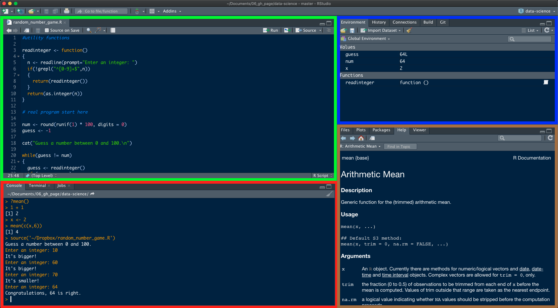
One of the advantages of using RStudio is that all the information you need to write code is available in a single window. Additionally, with many shortcuts, autocompletion and highlighting for the major file types you use while developing in R, RStudio will make typing easier and less error-prone. To get started, open RStudio just as you would open any other application on your computer. When you do, a window should appear in your screen like the one shown in the Figure below. RStudio is divided into 4 Panes.
At first startup you will not see an open script as seen in the green frame. You can create one by clicking first on ![]() (new file) and then on
(new file) and then on ![]() (new R script) in the upper left corner. Alternatively you can use the shortcut Shift+⌘+N on macOS or Shift+Ctrl+N on Windows & Linux.
(new R script) in the upper left corner. Alternatively you can use the shortcut Shift+⌘+N on macOS or Shift+Ctrl+N on Windows & Linux.
The basis of programming is that we write down instructions for the computer to follow, and then we tell the computer to follow those instructions. We write, or code, instructions in R because it is a common language that both the computer and we can understand. We call the instructions commands and we tell the computer to follow the instructions by executing (also called running) those commands. There are two main ways of interacting with R: by using the console or by using script files.
Console
> prompt for your next command. For example, if you type 10 * 10 and hit Enter, RStudio will display:> 10 * 10
[1] 100
>You’ll notice that a [1] appears next to your result. R is just letting you know that this line begins with the first value in your result. Some commands return more than one value, and their results may fill up multiple lines. For example, the command 1:100 returns 100 integer (numbers that have no digits after the decimal point). It creates a sequence of integers from 1 to 100. Notice that new bracketed numbers appear at the start of the second and third lines of output. These numbers just mean that the second line begins with the 18th value in the result, and the third line begins with the 35th value and so on. You can mostly ignore the numbers that appear in brackets:
  [1]   1   2   3   4   5   6   7   8   9  10  11  12  13  14  15  16  17
 [18]  18  19  20  21  22  23  24  25  26  27  28  29  30  31  32  33  34
 [35]  35  36  37  38  39  40  41  42  43  44  45  46  47  48  49  50  51
 [52]  52  53  54  55  56  57  58  59  60  61  62  63  64  65  66  67  68
 [69]  69  70  71  72  73  74  75  76  77  78  79  80  81  82  83  84  85
[86] 86 87 88 89 90 91 92 93 94 95 96 97 98 99 100: returns every integer between two integers. It is an easy way to create a sequence of numbers.If you type an incomplete command and press Enter, R will display a + prompt, which means R is waiting for you to type the rest of your command. This is because you have not closed a parenthesis or quotation, i.e. you do not have the same number of left-parentheses as right-parentheses, or the same number of opening and closing quotation marks. Either finish the command or hit Esc to start over:
> 99 +
+
+ 1
[1] 100
If you type a command that R doesn’t recognize, R will return an error message. If you ever see an error message, don’t panic. R is just telling you that your computer couldn’t understand or do what you asked it to do. You can then try a different command at the next prompt:
> 100 % 2
Error: unexpected input in "100 % 2"
>
Once you get the hang of the command line, you can easily do anything in R that you would do with a calculator. For example, you could do some basic arithmetic:
2 * 3
## 6

4 - 1
## 3

6 / (4 - 1)
## 2
Did you notice something different about this code? I’ve left out the >’s and [1]’s. This will make the code easier to copy and paste if you want to put it in your own console.
R treats the hashtag character # in a special way; R will not run anything that follows a hashtag on a line. This makes hashtags very useful for adding comments and annotations to your code. Humans will be able to read the comments, but your computer will pass over them. The hashtag is known as the commenting symbol in R.
For the remainder of the book, we’ll use hashtags to display the output of R code. We’ll use a single hashtag to add my own comments and a double hashtag ## to display the results of code. We’ll avoid showing > and [1] unless we want you to look at them.
Exercise
That’s the basic interface for executing R code in RStudio. Think you have it? If so, try doing these simple tasks to calculate the economic order quantity step by step with the given formula (Hint: Use sqrt(x) to calculate the square root).
$$Q = \sqrt{\frac{2DK}{h}}$$
Calulate the Q where:
$D = 1000$, $K = 5$, $h = 0.25$
Solution
# Step by step
2 * 1000 * 5
## 10000
10000 / 0.25
## 40000
sqrt(40000)
## 200
# Or as an one-liner
sqrt((2 * 1000 * 5) / 0.25)
## 200Throughout the course, I’ll put exercises in chunks, like the one above. I’ll follow each exercise with a hidden model answer, like the one above.
Source
RStudio allows you to execute commands directly from the script editor by using the Ctrl + Enter shortcut (on Macs, Cmd + Return will work, too). The command on the current line in the script (indicated by the cursor) or all of the commands in the currently selected text will be sent to the console and executed when you press the shortcut.
Exercise
Write your calculations for the EOQ in the script editor and …
- … execute a single line (click the Run icon
 or hit Cmd+Return). Note that the cursor can be anywhere on the line and one does not need to highlight anything (unless you want to define a function)
 - … execute multiple lines (Highlight lines with the cursor, then click Run or press Cmd+ Return
- … execute the whole script (Source icon
 or Cmd + Shift + S)
Note that running code via source differs in a few respects from entering it at the R command line. Sourcing a file does not print command outputs. To see your output click the arrow next to the source icon ![]() and click
and click Source with Echo or use Cmd + Shift + Return.
Objects / Assignment operator
You can get now output from R simply by typing math in the console or by running a script. You generated different numbers for you to see, but it didn’t save that values anywhere in your computer’s memory. If you want to use those numbers again, you’ll have to ask your computer to save them somewhere. You can do that by creating R objects. R lets you save data by storing it inside an R object. What is an object? Just a name that you can use to call up stored data. For example, you can save data into an object like a or b. Wherever R encounters the object, it will replace it with the data saved inside.
To create an object, we need to give it a name followed by the assignment operator <- (less-than symbol, followed by a minus sign), and the value we want to give it next to it. Typing ⌥ + - (mac) will write <- in a single keystroke. R ignores spaces and line breaks and executes one complete expression at a time. But it makes the code easier for you and me to read.
Q <- 200
die <- 1:6= for assignments, but not in every context. Because of the slight differences in syntax, it is good practice to always use <- for assignments.To see what is stored in an object, just type the object’s name by itself.
Q <- 200
Q
## 200

die <- 1:6
die
## 1 2 3 4 5 6
You can name an object in R almost anything you want such as x, current_temperature, or subject_id, but there are a few rules. First, a name cannot start with a number (2x is not valid, but x2 is). Second, a name cannot use some special symbols, like ^, !, $, @, +, -, /, or *. You want your object names to be explicit and not too long. There are some names that cannot be used because they are the names of fundamental functions in R (e.g. if, else, for, etc.). In general, even if it’s allowed, it’s best to not use other function names (e.g., c, T, mean, data, df, weights). It’s also best to avoid dots (.) within an object name as in my.dataset. There are many functions in R with dots in their names for historical reasons, but because dots have a special meaning in R (for methods) and other programming languages, it’s best to avoid them. It is also recommended to use nouns for object names, and verbs for function names. It’s important to be consistent in the styling of your code (where you put spaces, how you name objects, etc.). Using a consistent coding style makes your code clearer to read for your future self and your collaborators.
Exercise
Another important question here is, is R case sensitive? Is A the same as a? Figure out a way to check for yourself.
Environment
mtcars (this is a exemplary built in dataframe) to a name of your choice and take a look. Also in this pane is the History tab, where you can see all of the code executed for the session. You can also run history() to open it up. If you double-click a line or highlight a block of lines and then double-click those, you can send it to the Console (i.e., run them). The history will not be saved if we did not choose to save the environment after a session. The Build Tab will be useful later when you create your own website to hand in your code. We will come back to this shortly.Exercise
Now that we know how to put values into memory, we can do arithmetic with it and calculate EOQ again. Assign all values to R objects. Replicate the formula with those ojects, so that you just can run the line again even if another value changes.
Solution
D <- 1000
K <- 5
h <- 0.25
sqrt(2 * D * K / h)
## 200
D <- 4000
sqrt(2 * D * K / h)
## 400
Functions
R comes with many functions that you can use to do sophisticated tasks like random sampling. For example, you can round a number with the round() function, or as you have already done, calculate its square root with the sqrt() function. Using a function is pretty simple. Just write the name of the function and then the data you want the function to operate on in parentheses:
round(3.1415)
## 4

sqrt(16)
## 4
The data that you pass into the function is called the function’s argument. The argument can be raw data, an R object, or even the results of another R function. In this last case, R will work from the innermost function to the outermost. Here R first looks up die, then calculates the mean of one through six, then rounds the mean:
mean(1:6)
## 3.5

die <- 1:6
mean(die)
## 3.5

round(mean(die))
## 4
Many R functions take multiple arguments that help them do their job. You can give a function as many arguments as you like as long as you separate each argument with a comma.
round(3.1415)
## 3

round(3.1415, digits = 2)
## 3.14

sample(die, size = 1)
## 3
With the sample function you can simulate rolling a pair of dice, if you set the argument size to the value 2. But additonally, you have to set the value replacement to TRUE. Otherwise rolling pairs would not be possible. If you want to add up the dice, you can feed your result straight into the sum function:
dice <- sample(die, size = 2, replace = TRUE)
dice
## 3 4

sum(dice)
## 7
Writing your own function
You can now run this chunk again and again to simulate rolling the dice. However, this is an awkward way to work with the code. It would be easier to use your code if you wrapped it into its own function.
Every function in R has three basic parts: a name, a body of code, and a set of arguments. To make your own function, you need to replicate these parts and store them in an R object, which you can do with the function() function. To do this, call function() and follow it with a pair of braces, {}:
my_function <- function() {}function will build a function out of whatever R code you place between the braces. For example, you can turn your dice code into a function by calling:
roll <- function() {
  die <- 1:6
  dice <- sample(die, size = 2, replace = TRUE)
  sum(dice)
}To use it, write the object’s name followed by an open and closed parenthesis:
roll()
## 6
The code that you place inside your function is known as the body of the function. When you run a function in R, R will execute all of the code in the body and then return the result of the last line of code. If the last line of code doesn’t return a value, neither will your function, so you want to ensure that your final line of code returns a value.
What if you want to choose the kind of dice (number of sides of the die) each time you roll them? For that, you have to replace the object die, which indicates six faces, with another object:
roll2 <- function() {
  dice <- sample(faces, size = 2, replace = TRUE)
  sum(dice)
}

roll2()
## Error in sample(faces, size = 2, replace = TRUE) :
##   object 'faces' not found
Now you’ll get an error when you run the function. The function needs an object faces to do its job, but there is no object named faces to be found. You can supply faces when you call roll2() if you make faces an argument of the function. To do this, put the name faces in the parentheses that follow function when you define roll2:
roll2 <- function(faces) {
  dice <- sample(faces, size = 2, replace = TRUE)
  sum(dice)
}

roll2(faces = 1:6)
## 7

roll2(faces = 1:10)
## 13
Notice that roll2() will still give an error if you do not supply a value for the faces argument when you call roll2(). You can prevent this error by giving the faces argument a default value. To do this, set faces equal to a value when you define roll2():
roll2 <- function(faces = 1:6) {
  dice <- sample(faces, size = 2, replace = TRUE)
  sum(dice)
}

roll2()
## 9
Exercise
What if you also want to choose the number of dice each time you roll them? Try to alter the function accordingly. Set the default value to 2 dice.
Solution
roll2 <- function(faces = 1:6, number_of_dice = 2) {
dice <- sample(x = faces, size = number_of_dice, replace = TRUE)
sum(dice)
}
roll2()
## 10
# Four Tetrahedron shaped dice (Four faces)
roll2(faces = 1:4, number_of_dice = 4)
## 11Exercise
Now transfer that approach to the EOQ formula and create a function, which calculates the EOQ and takes the variable D as an argument (set the default value of D to 1000)!
Solution
calc_EOQ <- function(D = 1000) {
K <- 5
h <- 0.25
Q <- sqrt(2*D*K/h)
Q
}
calc_EOQ()
## 200
calc_EOQ(D = 4000)
## 400Miscellaneous
Files tab has a navigable file manager, just like the file system on your operating system. It shows all the files and folders in the default workspace. The Plot tab is where graphics you create will appear. Here we can zoom, export, configure and inspect graphs/figures. Run hist(mtcars$mpg) for an example. The Packages tab shows you the packages that are installed and those that can be installed (more on this later). The Help tab allows you to search the R documentation for help and is where the help appears when you ask for it from the Console.Getting help
Within RStudio
There are over 1,000 functions at the core of R, and new R functions are created all of the time. This can be a lot of material to memorize and learn! Luckily, each R function comes with its own help page, which you can access by typing the function’s name after a question mark. For example, each of these commands will open a help page. Look for the pages to appear in the Help tab of RStudio’s bottom-right pane:
?sqrt
?log10
?sample
Help pages contain useful information about what each function does. These help pages also serve as code documentation, so reading them can be bittersweet. They often seem to be written for people who already understand the function and do not need help.
Don’t let this bother you—you can gain a lot from a help page by scanning it for information that makes sense and glossing over the rest. This technique will inevitably bring you to the most helpful part of each help page: the bottom. Here, almost every help page includes some example code that puts the function in action. Running this code is a great way to learn by example.
Parts of a Help Page
Each help page is divided into sections. Which sections appear can vary from help page to help page, but you can usually expect to find these useful topics:
Description - A short summary of what the function does.
Usage - An example of how you would type the function. Each argument of the function will appear in the order R expects you to supply it (if you don’t use argument names).
Arguments - A list of each argument the function takes, what type of information R expects you to supply for the argument, and what the function will do with the information.
Details - A more in-depth description of the function and how it operates. The details section also gives the function author a chance to alert you to anything you might want to know when using the function.
Value - A description of what the function returns when you run it.
See Also - A short list of related R functions.
Examples - Example code that uses the function and is guaranteed to work. The examples section of a help page usually demonstrates a couple different ways to use a function. This helps give you an idea of what the function is capable of. You can also type example(function_name)to get examples for said function.
If you’d like to look up the help page for a function but have forgotten the function’s name, you can search by keyword. To do this, type two question marks followed by a keyword in R’s command line. R will pull up a list of links to help pages related to the keyword. You can think of this as the help page for the help page:
??logExternal to RStudio
R also comes with a super active community of users that you can turn to for help. Stack Overflow, a website that allows programmers to answer questions and users to rank answers based on helpfulness, is the best place to find an answer to your question. You can submit your own question or search through Stack Overflow’s previously answered questions related to R, because there’s a great chance that your question has already been asked and answered. You’re more likely to get a useful answer if you provide a reproducible example with your question. This means pasting in a short snippet of code that users can run to arrive at the bug or question you have in mind.
Addtionally to Stackoverflow you can just use google.com or rseek.org to search for an r related problem.
Exercise
Find a way to alter the probabilities involved in the sampling process, if your roll one die. Let’s change the probability of rolling a 6 to 50% (Because the probabilites need to sum one, the other faces have a probability of 10%). Start by opening the help page of the function sample() and take a look at the arguments.
Hint: You can create a vector with the c() function. For example:
probabilities_vector <- c(1/6, 1/6, 1/6, 1/6, 1/6, 1/6)
probabilities_vector
## 0.1666667 0.1666667 0.1666667 0.1666667 0.1666667 0.1666667
Solution
roll3 <- function(faces = 1:6, number_of_dice = 1) {
  dice <- sample(x = faces, size = number_of_dice,
                            replace = TRUE,
                            prob = c(0.1, 0.1, 0.1, 0.1, 0.1, 0.5))
  sum(dice)
}
# You can run the function 100 times, store the results and plot a histogram to varify your function
results <- replicate(n = 100, expr = roll3(), simplify=TRUE)
hist(results)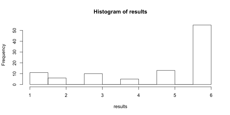
Datacamp
Mattermost
In the course of the next chapters, we will do a lot of coding and it is very likely that errors will occur. That can have several reasons but dealing with errors is an elementary component in programming in data science and machine learning. As already mentioned, in the most cases other people from around the world have had similar problems and you will find the right solution to your problem performing a query on the internet. Please try to do that as a first step when you run into an error.
If you don’t find a solution and feel you are stuck, don’t hesitate to use the relevant Mattermost channel. For each chapter there will be a channel where we try to help you as much as possible. But in order to keep it efficient and manageable it is necessary that we all follow some basic rules:
- Use the right channel: for each chapter there is a correct channel as well as a general channel for questions that do not relate to a specific chapter.
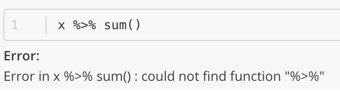
- Post error message: if you run into an error it is necessary that we know what the error is. Often reading the error message very carefully can also help you to understand where the problem comes from.
- Post the code that caused the error: in order to reproduce the error we need the last command that caused the error. If we need more context we will ask you for that.
- Use the formatting guidelines of Mattermost when you post code. That makes a huge difference in terms of readability. They will also be linked in the channel description. Most important is that using ``` one line above and one line below your code will make it easy to read.
- Use thread function to reply to a discussion. This way a discussion can be easier read. You find the reply button on the right side of a message.
- Use the search function: It will allow you to search across channels for similar problems as it is very likely that the you encounter the same problems as the other students.
Playing by these rules makes it a lot easier for everyone to follow the discussion and learn from similar problems and everyone can benefit from the discussions.
```r
x %>% sum()
```

**Error:**
Error in x %>% sum() : could not find function "%>%"
GitHub for journaling
We will use GitHub to store your data and hand in your assignments through your personal website (github pages). To be able to do so, complete the following steps (detailed instructions below):
- Create a free github account (if you do not have one already).
- Download, install github desktop and connect it with your account. GitHub Desktop is a graphical user interface, which allows you to sync your local code changes with your online repository (if you are already familiar with git and github you might not need it).
- Check for git: You should already have git on your device, but let’s check for it anyway.
- Open RStudio
- In the Terminal, run the following command:
which git - If after running that you get something that looks like a file path to git on your computer, then you have git installed. For example, that might return something like this (or it could differ a bit): /usr/local/bin/git. If you instead get no response at all, you should download & install git from here: git-scm.com/downloads
- Accept the assignment on GitHub Classroom, create a website using Quarto and host it on Github pages, then submit the link and your personal password to your website for the assignments. You will create the website using this template Journal Data Science. You can open it using the password: test.
To get started with this template you only have to login to github and click this invitation link:
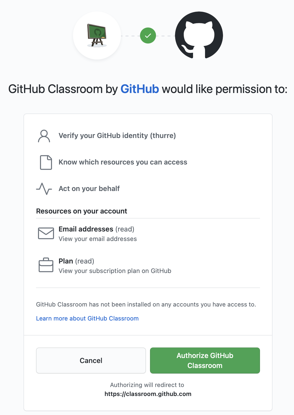
Authorize GitHub Classroom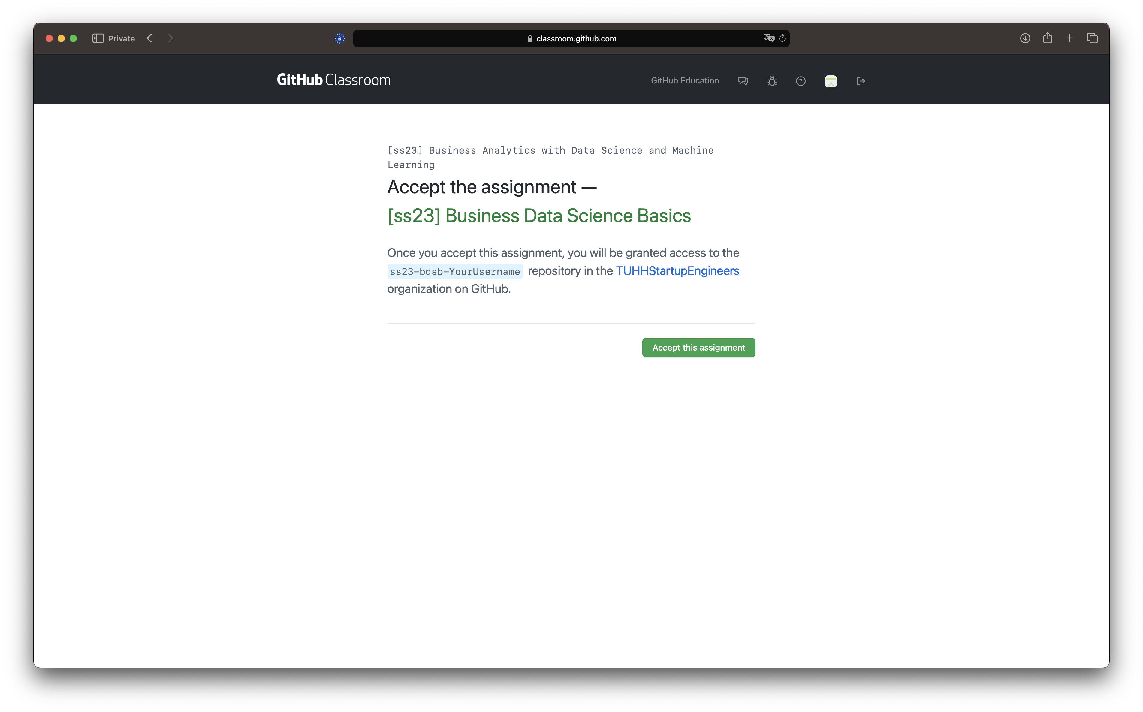
Accept Assignment …
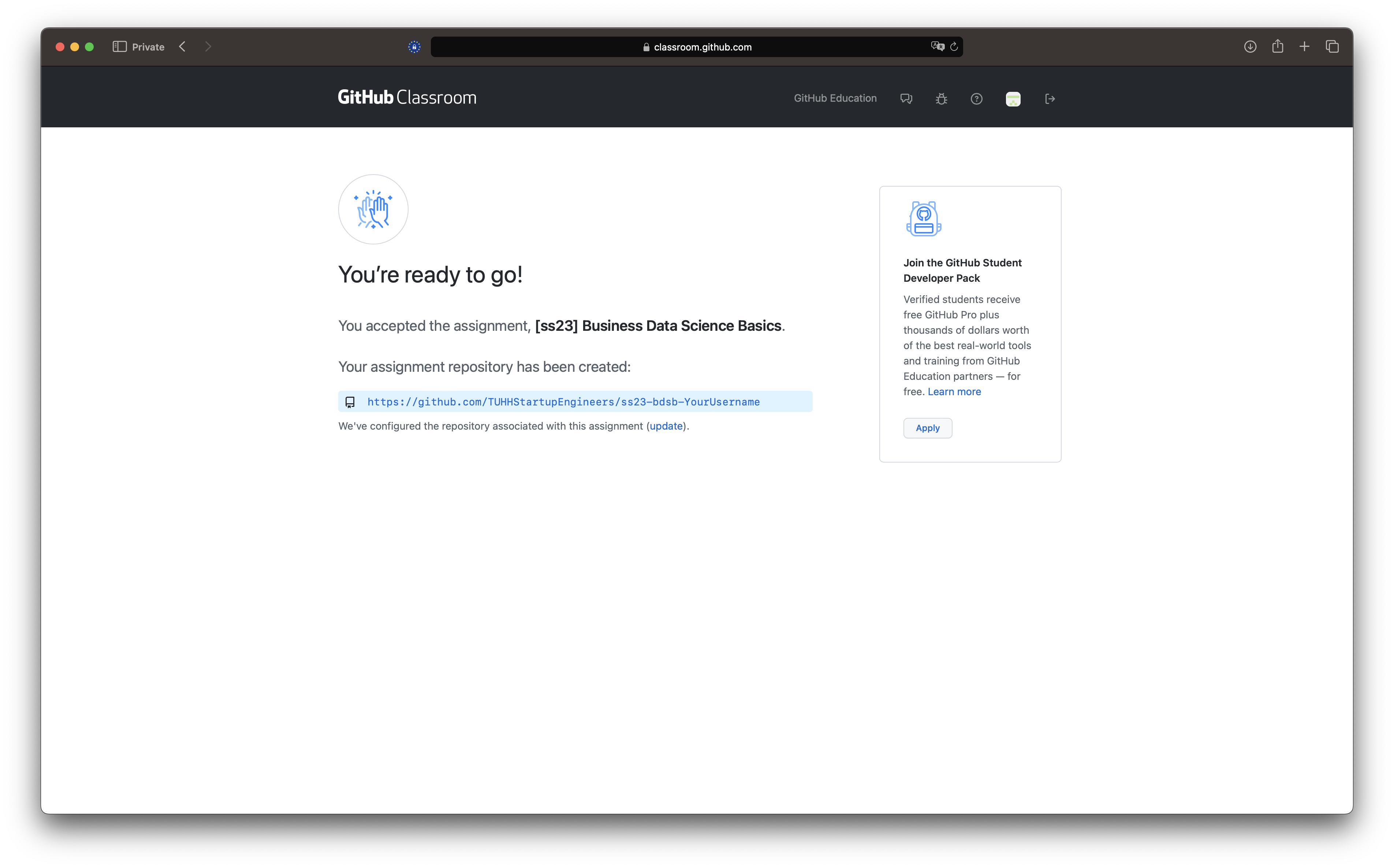
You might have to refresh the page after a while. But then you’re ready to go and able to access your template by clicking on the bottom link (you don’t need to accept the invitation to TUHHStartupEngineers). That means you have all of the files you need to compile a website with Quarto.
Compiling on your local computer
Make sure the
rmarkdownpackage and all it’s dependencies are installed in RStudio: Open RStudio, click the packages tab in the lower right hand corner, click install packages, type inrmarkdown, make sure “install dependencies” is clicked on, then press install (alternatively runinstall.packages("rmarkdown", dependencies = TRUE)in the console).Only necessary if you do not have the most recent version of RStudio installed: Install Quarto
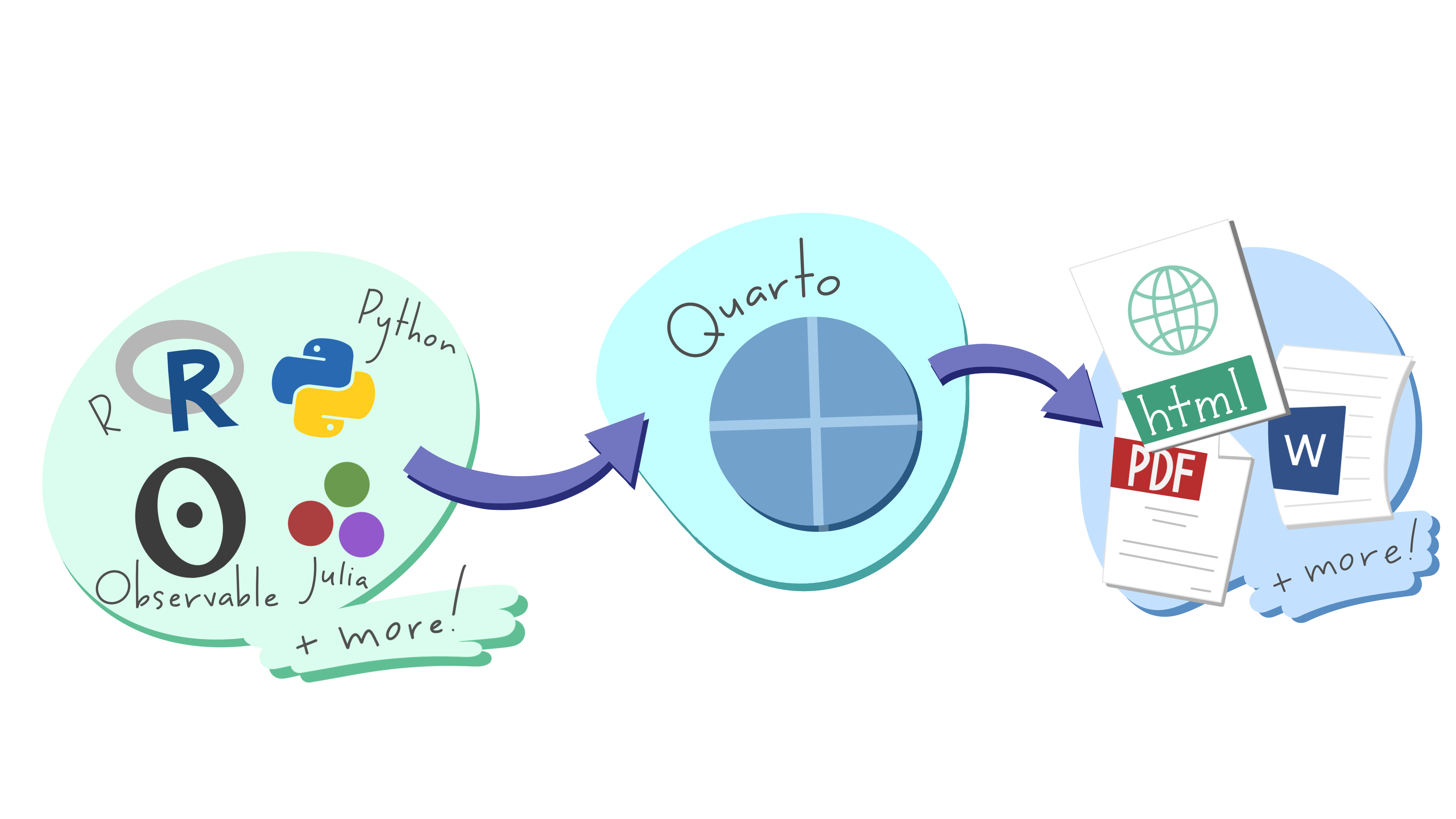
What is Quarto? Quarto is a scientific publishing tool built on Pandoc that allows R, Python, Julia, and ObservableJS users to create dynamic documents, websites, books and more.
Quarto is now included with RStudio v2022.07.1+ so no need for a separate download/install if you have the latest version of RStudio!
Quarto will work with RStudio v2022.02+, but you’ll need to install Quarto separately here (we recommend just installing the most up to date version of RStudio).
macOS only: Install the Apple Xcode developer tools.
- Option 1: Run
xcode-select --installin the terminal.
You can copy commands directly in your terminal (Terminal on MacOS, Command Prompt on Windows).
- Option 2: You can install Xcode for free from the App Store.
Windows only: Download and install the latest version of Rtools.
- Open GitHub Desktop, make sure it is connected to your account and clone your assignment repository to your computer so that you have a local copy of that data that was provided to you:

Sign in to GitHub.com
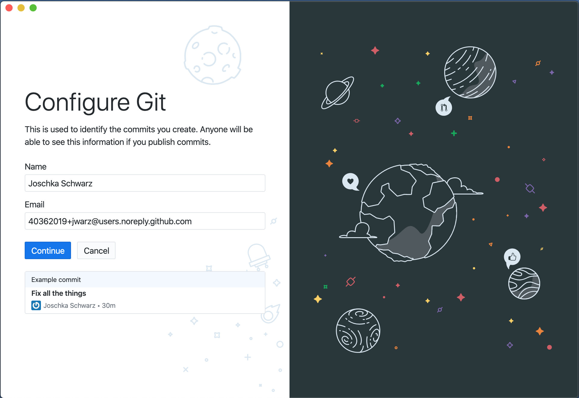
Continue)
Finish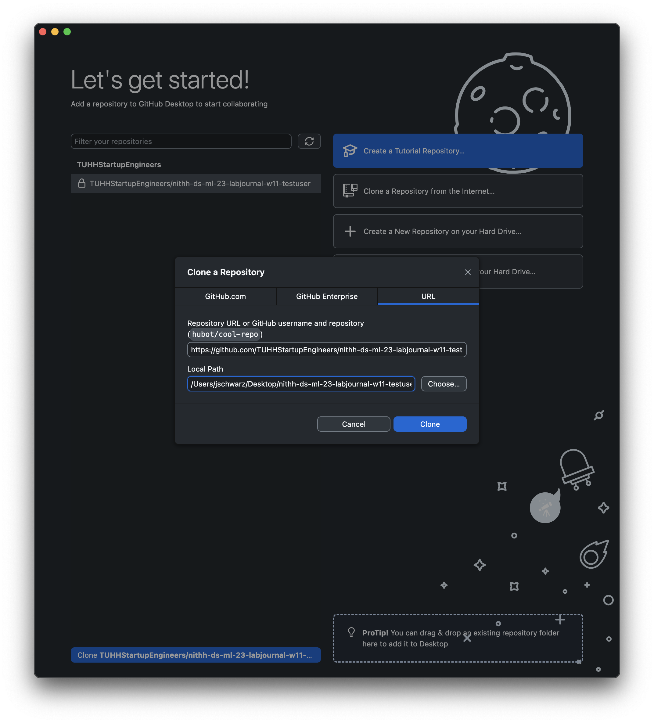
Clone a TUHHStartupEngineers/... in the bottom left or Add and then Clone Repository ... and select your TUHHStartupEngineers/...-YourUserName repo. Choose a local path where you want to save the local copy and press Clone.Navigate to the folder you just cloned/downloaded, open the
lab_journal.Rprojfile. This should automatically open RStudio, and your current working environment will be inside this project. That means everything you save will be auto saved to this folder (unless you tell RStudio to save something somewhere else. Have a look at the files tab in the bottom right hand corner. Most files you click will be opened up as text files in the RStudio editor. For each chapter there is a journal you should open and edit. If you save the file your website changes as well.To compile the entire website, find the build tab in the top right hand corner. You should see the option to
Render website Click this. The website should be built. After the website is built, you should be able to see it in the RStudio browser (viewer pane in the bottom right corner). There is a little button
  that allows you to pop the website into your default web-browser. This way you can look at the website in your browser.
Important: After compilation, all of the files for displaying your website are saved in the folder where your R project resides. When you look at these in a browser (for example, by going to the folder and dragging the _site/index.html file into a browser - don’t worry about the password protection for now), you are loading from your disk. Only you will be able to see the website, because it is on your hard-drive. You need to upload to a web server to serve the webpage on the internet.
that allows you to pop the website into your default web-browser. This way you can look at the website in your browser.
Important: After compilation, all of the files for displaying your website are saved in the folder where your R project resides. When you look at these in a browser (for example, by going to the folder and dragging the _site/index.html file into a browser - don’t worry about the password protection for now), you are loading from your disk. Only you will be able to see the website, because it is on your hard-drive. You need to upload to a web server to serve the webpage on the internet.
Serving your webpage on the internet
Every Github repository has the capability of serving html files (web page files) contained in the repository, this is called github pages. How this works depends a little bit on the specific repository you are using. For this repository the webpage is built into the _site folder and then served from the gh-pages branch. Your files contain a workflow (GitHub Action) that realizes all these steps. We only have to tell GitHub that the page is being built and served like this.
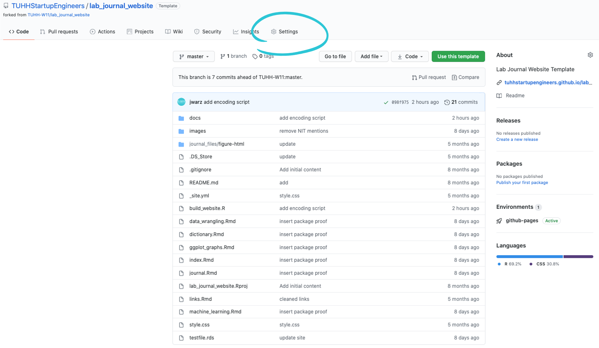
- Go to github.com, navigate to your journal repository (located in our account: https://github.com/TUHHStartupEngineers/...-YourUserName) and click the settings button in the top right corner.
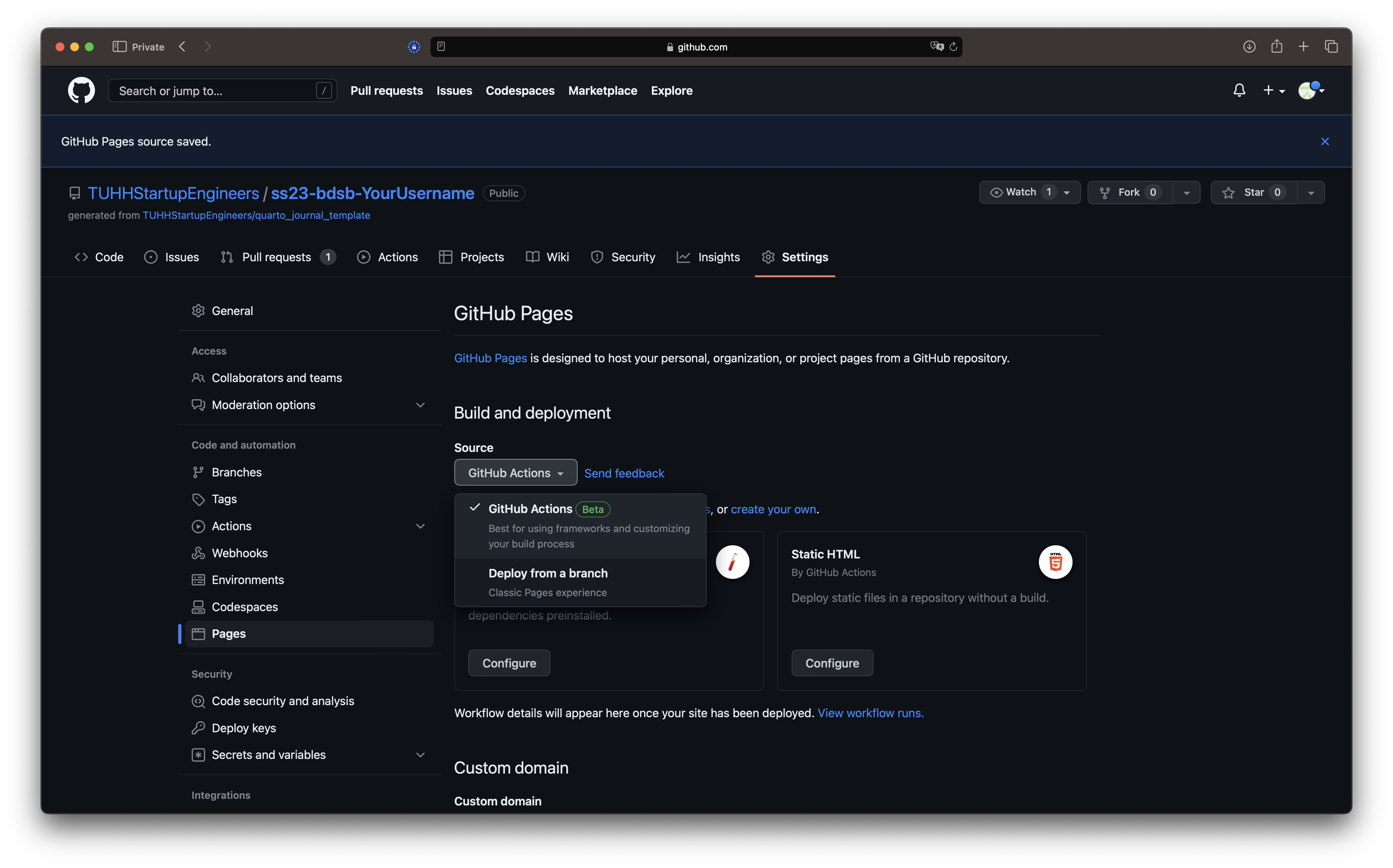
- Select
Pagesin the menu on the left and make sure the source GitHub Actions is set.
This Action requires a encrypted secret, which is basically the password to your website.
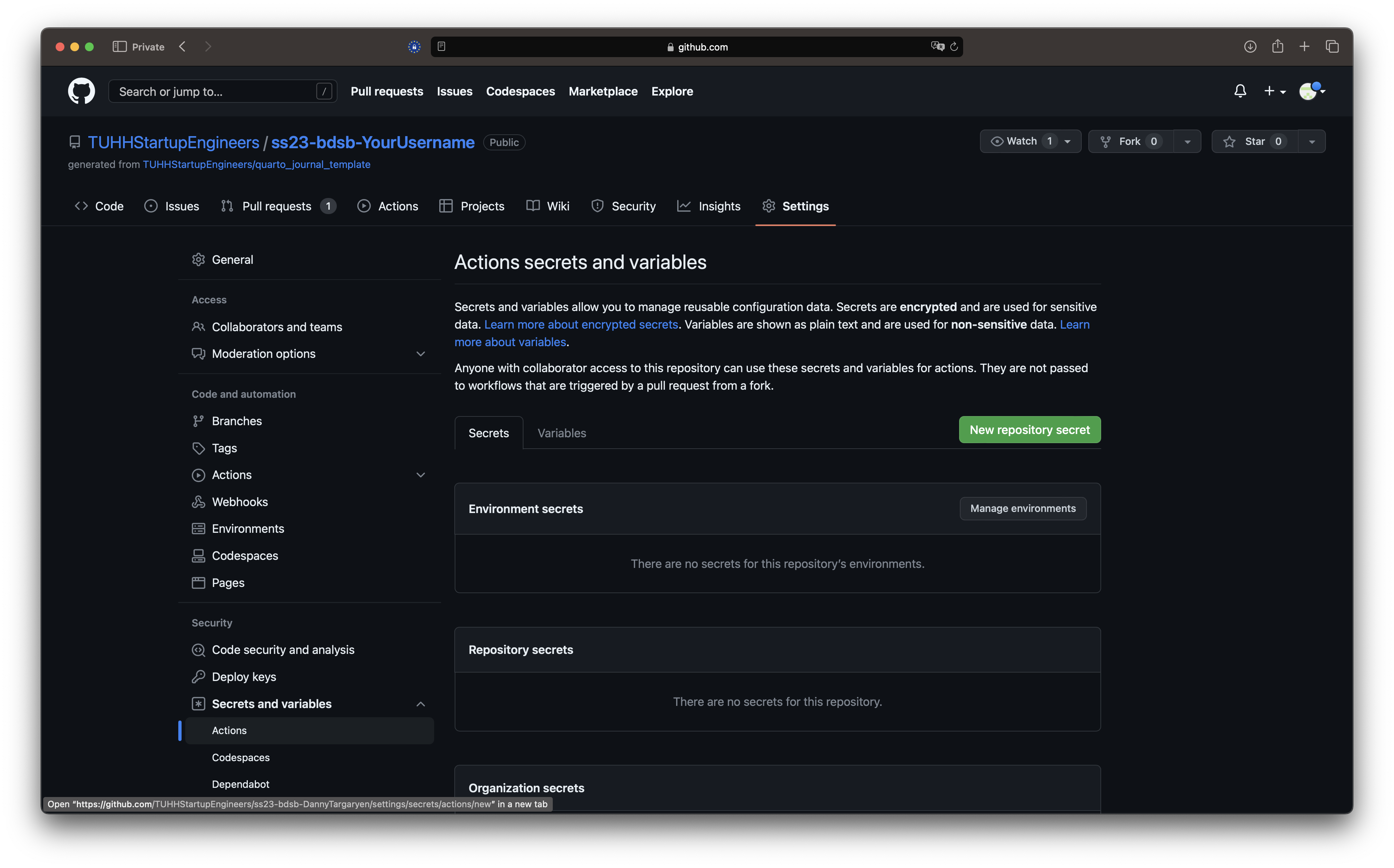
- Select
Secrets and variables->Actionsin the menu on the left. ClickNew repository secret
- The Name has to be
WEBSITE_TOKEN. The value for secret will be your password for your website. DO NOT USE YOUR STANDARD PASSWORDS. You later will be asked to submit your passwords to the teaching assistants who will be able to see it in clear text.
The website will be built and served every time you upload any new local changes to GitHub. Remember to render the website in RStudio every time you want to add changes to your site. For the first change open the index.qmd in RStudio and change the author name at the top. Then render the site again.
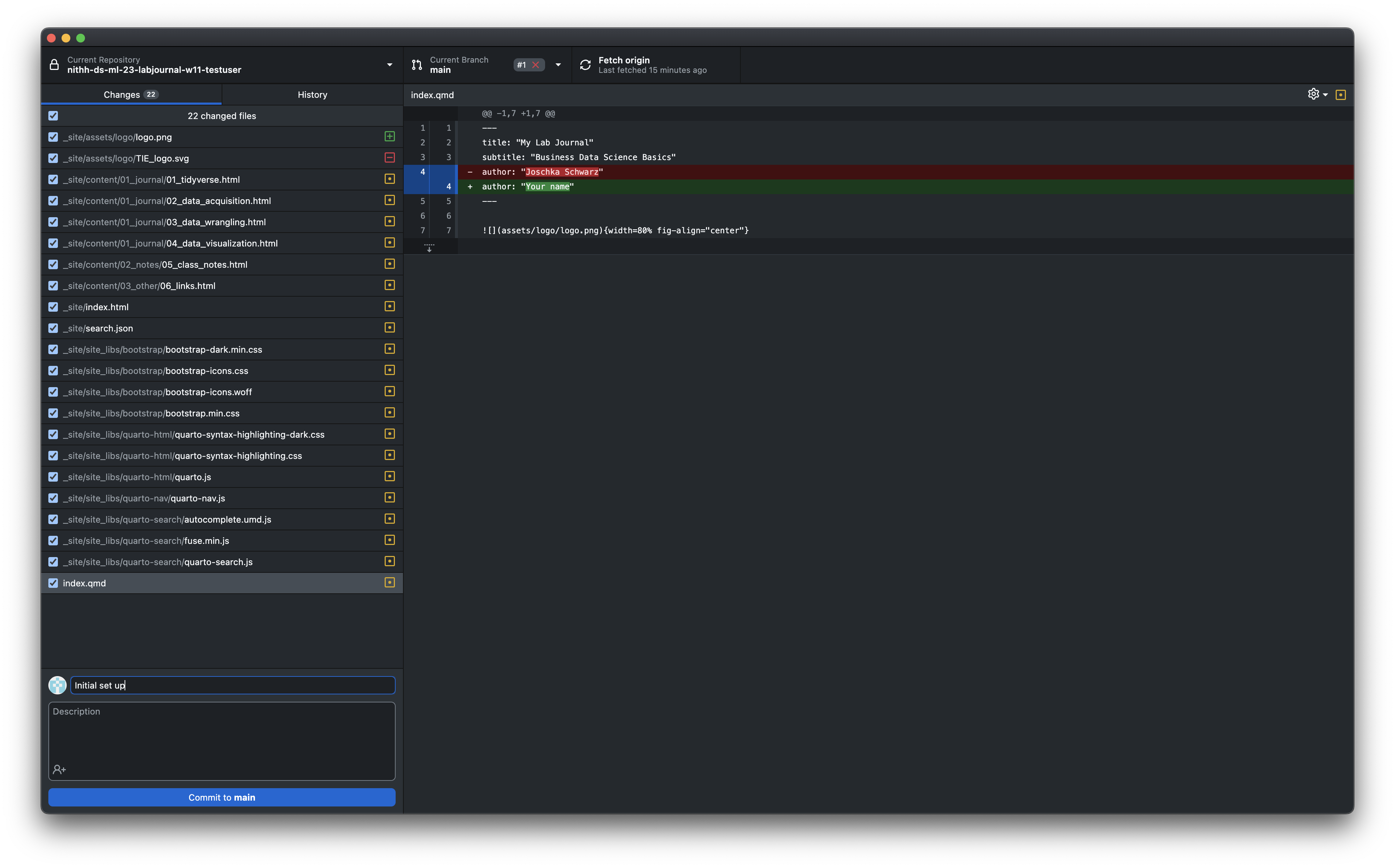
- To upload any changes to your content (e.g. the author name or the date in the
index.qmdfile) you have to commit your changes to github using github dektop (if you are familiar with git you are free to use another method to commit your changes). As shown in this Figure you see that GitHub Desktop detects the changes automatically after saving your files (don’t forget to build your website again after any changes. Otherwise the html files won’t be affected by any changes to your .qmd-files). Select all of the files that you want to commit on the left panel. Write a short note to describe the changes in the box at the bottom left. PressCommit to main.
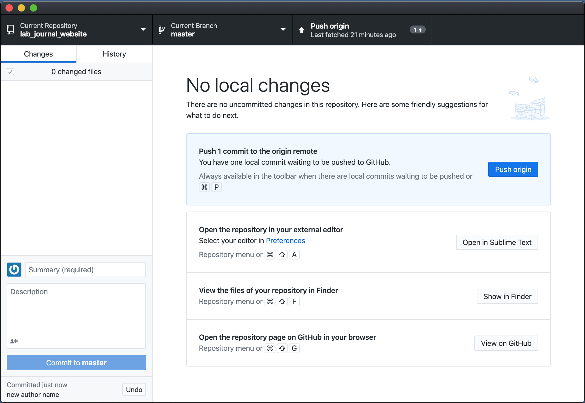
- Press
Push originand wait a couple of minutes. Your changes should now be served on your website
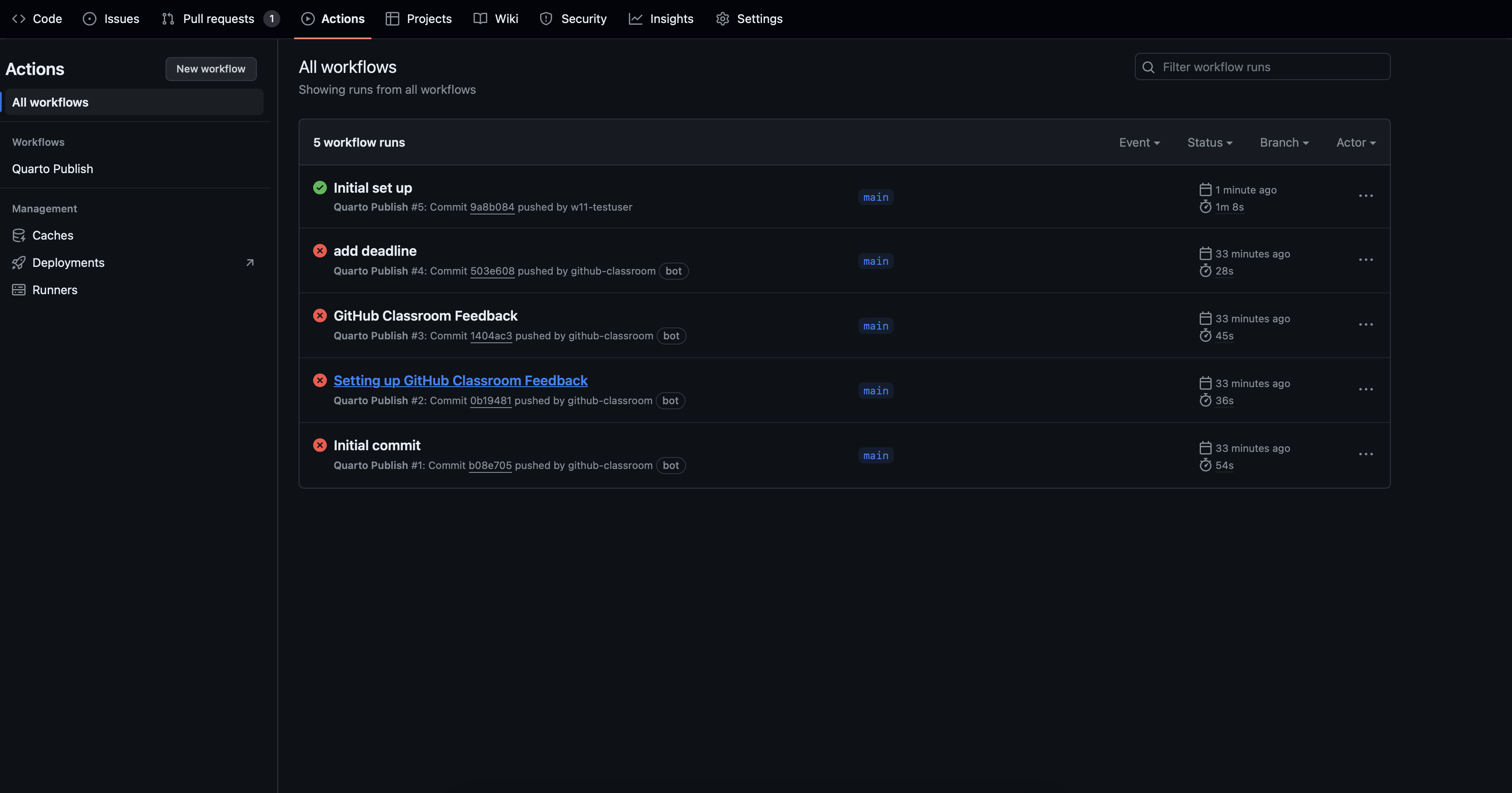
The process of building the website can be viewed in the Action Tab by clicking on your named commit.
Initial Set Up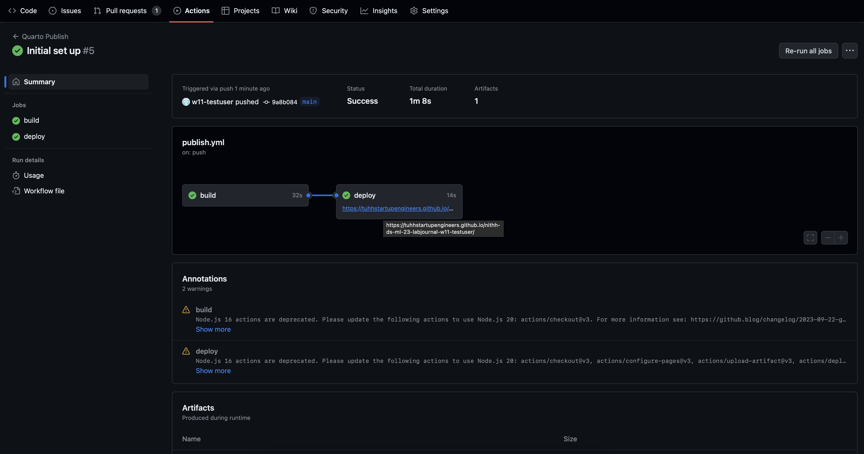
To avoid to enter your password every time you open your site or swich in between pages, set a checkmark at Remember Me below the password prompt.
Quarto
Quarto is a publishing system built on Pandoc that allows users to create dynamic content using R, Python, Julia, and ObservableJS (with plans to add more languages too!). R users have long loved RMarkdown for combining prose, code, and outputs into single “knitted” documents. Quarto extends all of RMarkdown’s best features (plus many more!) to additional languages.
You can explore Quarto’s documentation to learn more about creating documents, websites, blogs, books, slides, etc.
Each page of your website is created by a q-Markdown file (.qmd). This format resembles an earlier yet another markdown format, .Rmd, also managed by RStudio, but tries to abstract away from the original R basis of .Rmd.
All website pages are plain text file that have the extension .qmd. Notice that the file contains three types of content:
- An (optional) YAML header surrounded by - - - at the top (there is no need in the beginning to alter it)
- R code chunks surrounded by
```s. These chunks can be customized withknitroptions, arguments set at the top of a chunk header after #|:#| eval: falseprevents running the code and include its results#| include: falseprevents code and results from appearing in the finished file. Quarto still runs the code in the chunk, and the results can be used by other chunks.#| echo: falseprevents code, but not the results from appearing in the finished file. This is a useful way to embed figures.#| message: falseprevents messages that are generated by code from appearing in the finished file.#| warning: falseprevents warnings that are generated by code from appearing in the finished.#| fig-cap: "..."adds a caption to graphical results.
Example:
```{r}
#| eval: false
numbers <- 1:1000

# This will print the first 10 elements of the vector numbers
numbers[1:10]

# This will plot a histogram of 100 random elements of the vector numbers
hist(sample(numbers, 100, replace = T))
```
Check for yourself what happens, if you set eval to true.
- text mixed with simple text formatting
See the Quarto Cheat Sheet or the official quarto documentation for further information regarding the markdown syntax. It is necessary, that your code is formatted correctly to be evaluated.
Submission
Submit your journal URL and password via the following form. If you do not submit your information, we won’t be able to evaluate your assignments.
Datacamp
No quarto video available yet. But studying R Markdown definitely helps.